Data sets

The various ozone profile data records used by the LOTUS team during Phase 1 and Phase 2 can be made available upon request. Please contact the activity leaders.

LOTUS time series analysis codes

The LOTUS team uses a Multiple Linear Regression (MLR) analysis tool implemented in Python by the University of Saskatchewan, to infer long-term trends in ozone profile data sets. This code is freely available.

Dynamical Linear Modelling (DLM) offers an alternative approach to MLR. An implementation by Dr. J. Alsing can be downloaded freely from Github. Further information can be found in Alsing (2019). dlmmc: Dynamical linear model regression for atmospheric time-series analysis. Journal of Open Source Software, 4(37), 1157, https://doi.org/10.21105/joss.01157.

Logo LOTUS

	white background low-res .png | high-res .png
	black background low-res .png | high-res .png
	transparent, for light backgrounds low-res .png | high-res .png
	transparent, for dark backgrounds low-res .png | high-res .png

Figures LOTUS Report (2019)

Figures from this Report are in the public domain and may be used with proper attribution to source. Please use the following citation

Jump to... Executive Summary (1 figure) | Chapter 2 (6 figures) | Chapter 3 (19 figures) | Chapter 4 (11 figures) | Chapter 5 (14 figures) | Supplement (27 figures)

Executive Summary

Figure ES.1 | high-res .png Overview of ozone profile trends from past and recent assessments: WMO (2014), Harris et al. (2015), Steinbrecht et al. (2017), and LOTUS (this work) are shown in red, orange, blue, and black respectively. Top row shows trends before the turnaround of ODSs and bottom row since the turnaround (analysis time period differs by assessment). Shaded area and error bars represent the 95 % confidence interval for the combined trend. Coloured profiles are slightly offset on the vertical axis for display purposes...

Chapter 2

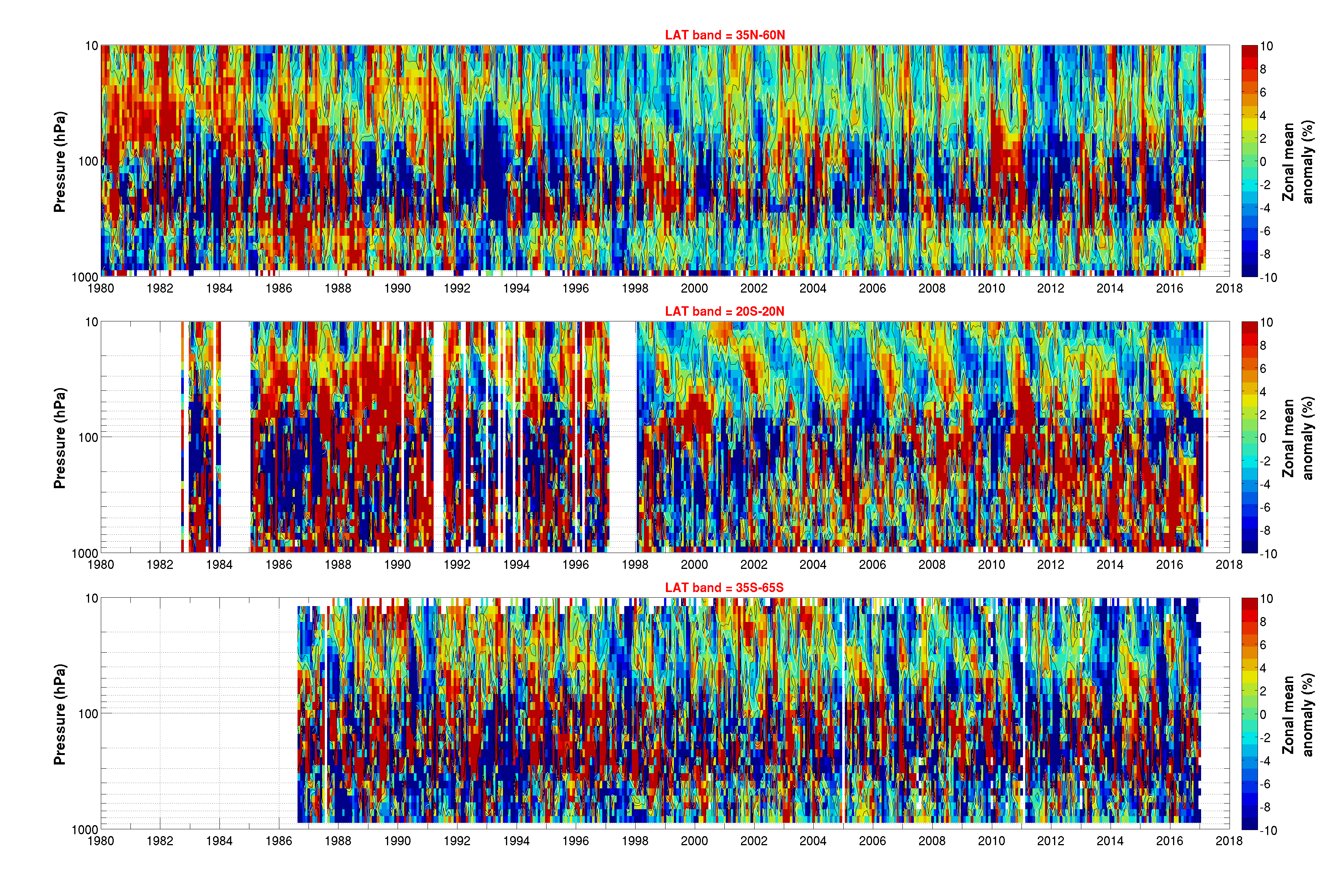	Figure 2.1 | high-res .png Example time series of monthly zonal mean relative deseasonalised anomalies computed from ozonesonde data in the 35°N–60°N (top), 20°S–20°N (centre), and 60°S–35°S (bottom) latitude bands as a function of altitude (ground to ~30 km).
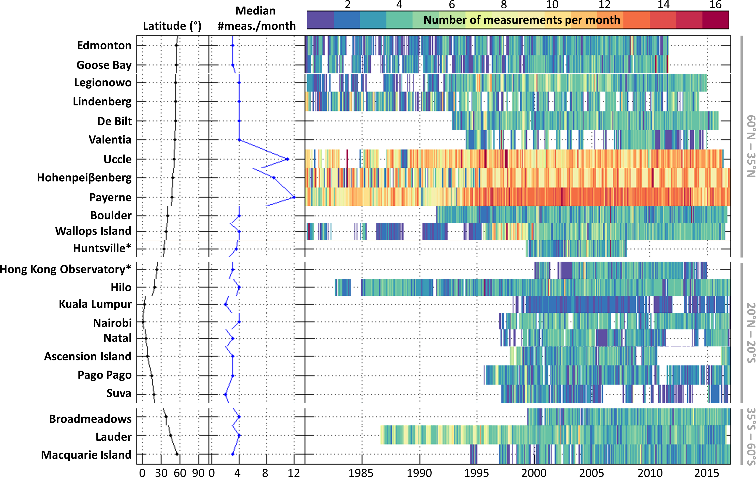	Figure 2.2 | high-res .png Sampling statistics for ozonesonde station records retrieved from the NDACC, WOUDC, and SHADOZ data archives, sorted North to South. The figure shows the median number of measurements per month over the entire data record (centre) and the number of measurements for each month since 1980 (right, colour scale). Stations with an asterisk are located slightly outside the attributed latitude zones.
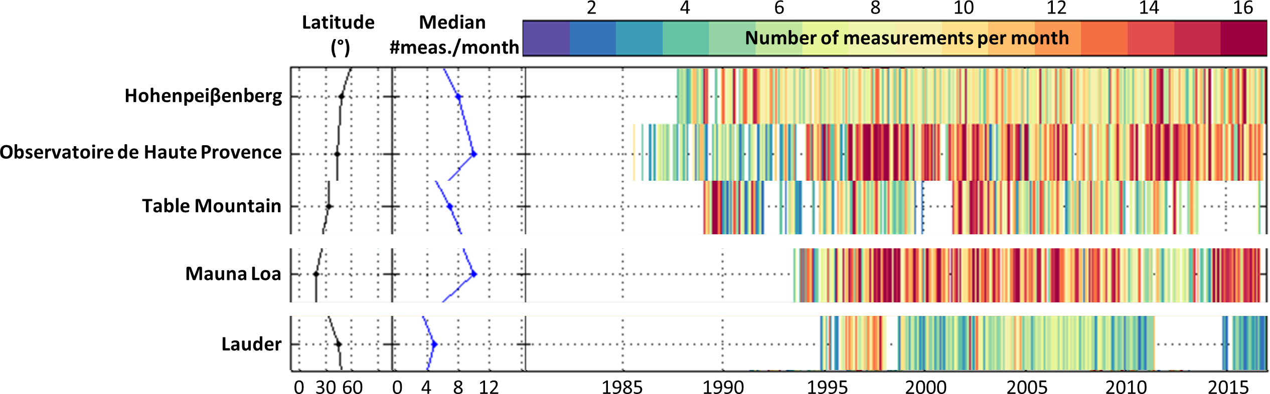	Figure 2.3 | high-res .png As Figure 2.2 but for the stratospheric ozone lidar station records retrieved from the NDACC data archive.
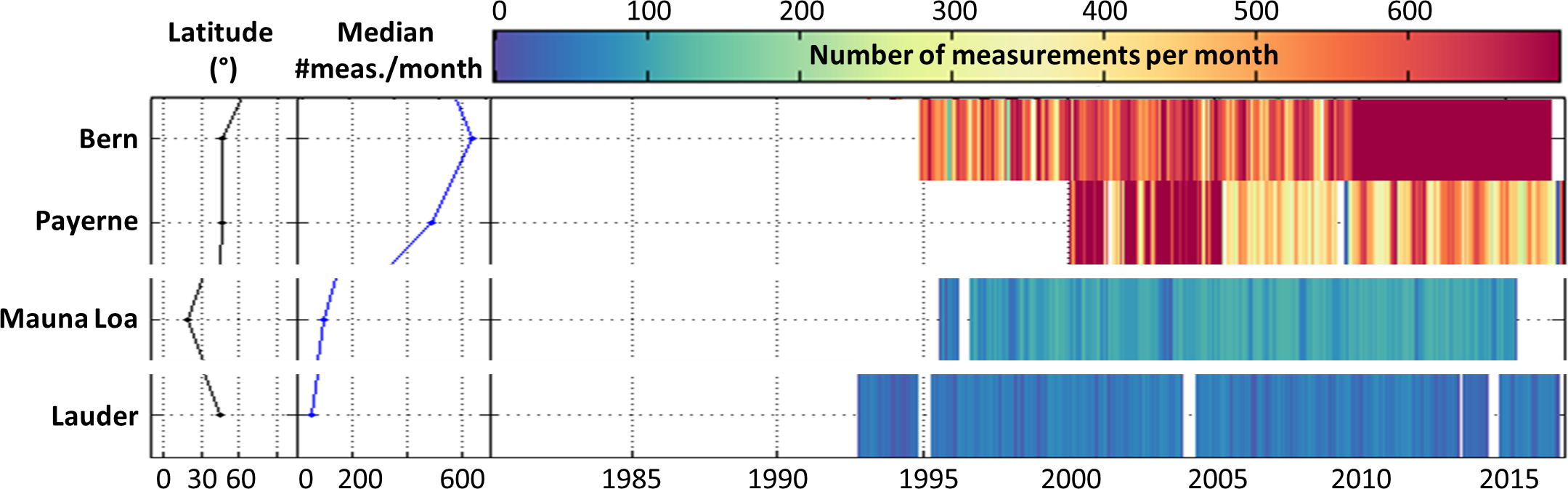	Figure 2.4 | high-res .png As Figure 2.2 but for ozone microwave radiometer station records retrieved from the NDACC data archive. Stations report half hourly, hourly, or six-hourly profiles.
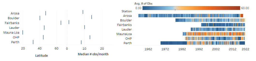	Figure 2.5 | high-res .png As Figure 2.2 but for Dobson Umkehr station records submitted by the record PIs to the LOTUS data archive. Stations report profiles once or twice a day. Note that the time axis differs from that of previous figures.
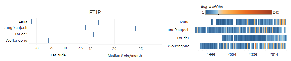	Figure 2.6 | high-res .png As Figure 2.2 but for FTIR station records submitted by the record PIs to the LOTUS data archive. Stations report profiles several times per day. Note that the time axis differs from that of previous figures.

Chapter 3

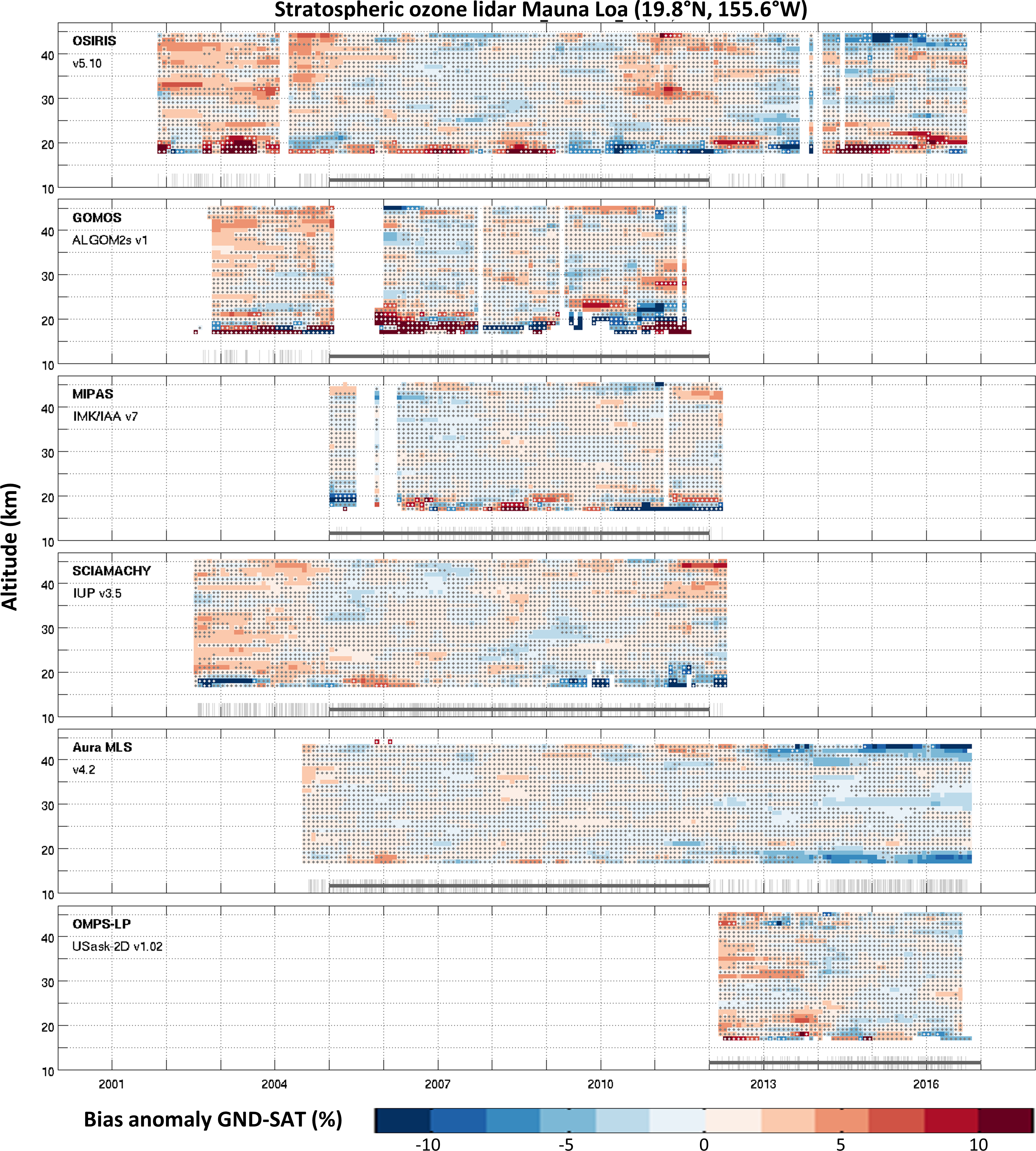	Figure 3.1 | high-res .png Smoothed anomaly time series (δ, see Eq. 3.1) of the relative difference of MLO lidar and six satellite ozone profile data records (top to bottom). Red values indicate regions in which lidar measurements are biased more positive (or less negative) compared to satellite than their median value during the reference period. Stippled areas denote δ values that are not statistically different from zero at the 2-sigma level. A running average with a 12-month window was used to smooth the time series. Thin grey vertical lines show the sampling of the co-located profile data records; the grey horizontal lines indicate the reference period for each comparison. Adapted from Hubert et al. (2019).
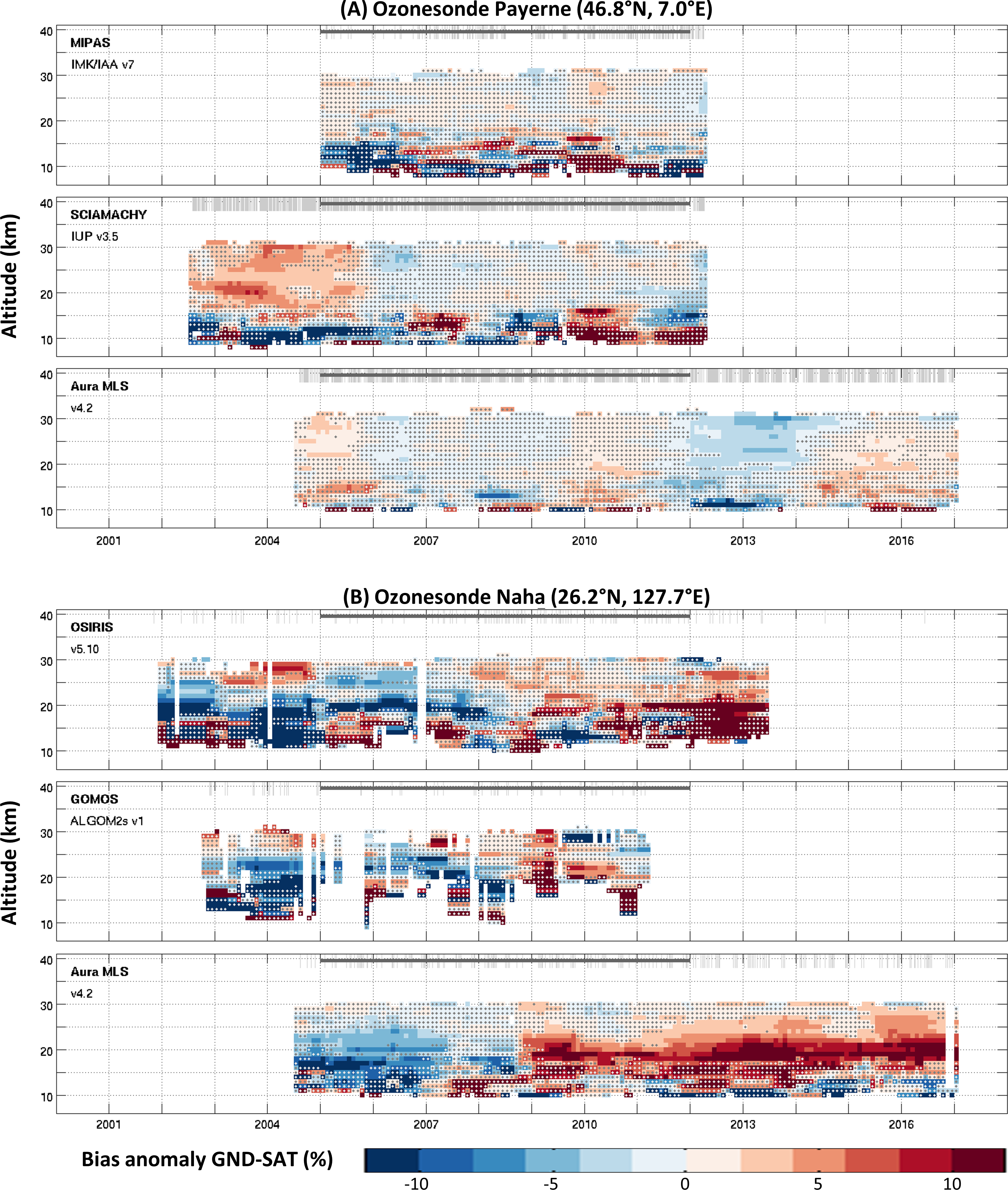	Figure 3.2 | high-res .png As Figure 3.1 but for two ozonesonde sites each with a different selection of three satellite references. Stippled areas denote non-significant δ values. Comparisons to all six satellite records for both stations are shown in Figures S3.1 and S3.2 in the Supplement. Adapted from Hubert et al. (2019).
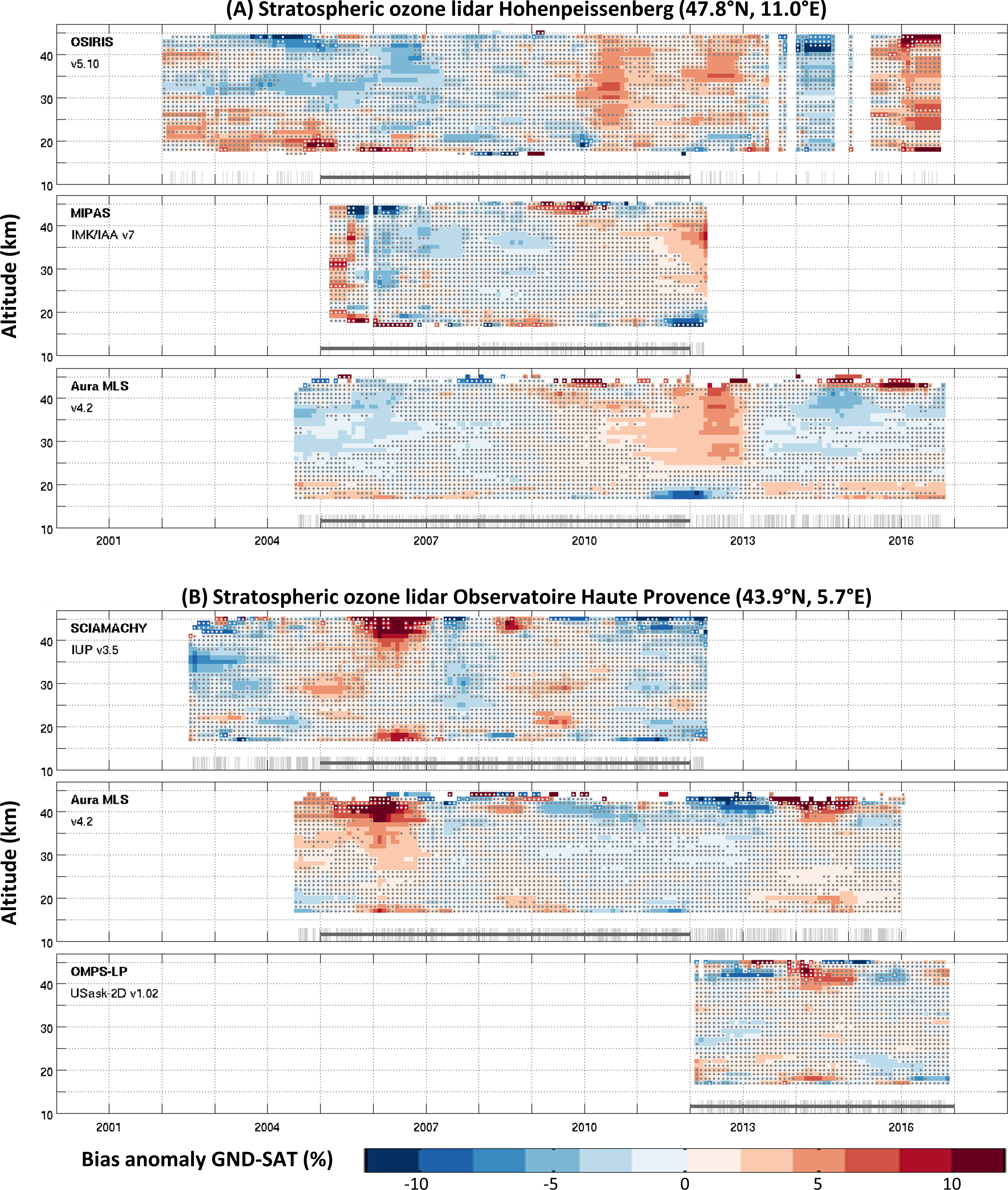	Figure 3.3 | high-res .png As Figure 3.2 but for two stratospheric ozone lidar sites. Stippled areas denote non-significant δ values. Comparisons to all six satellite records for both stations are shown in Figures S3.3 and S3.4 in the Supplement. Adapted from Hubert et al. (2019).
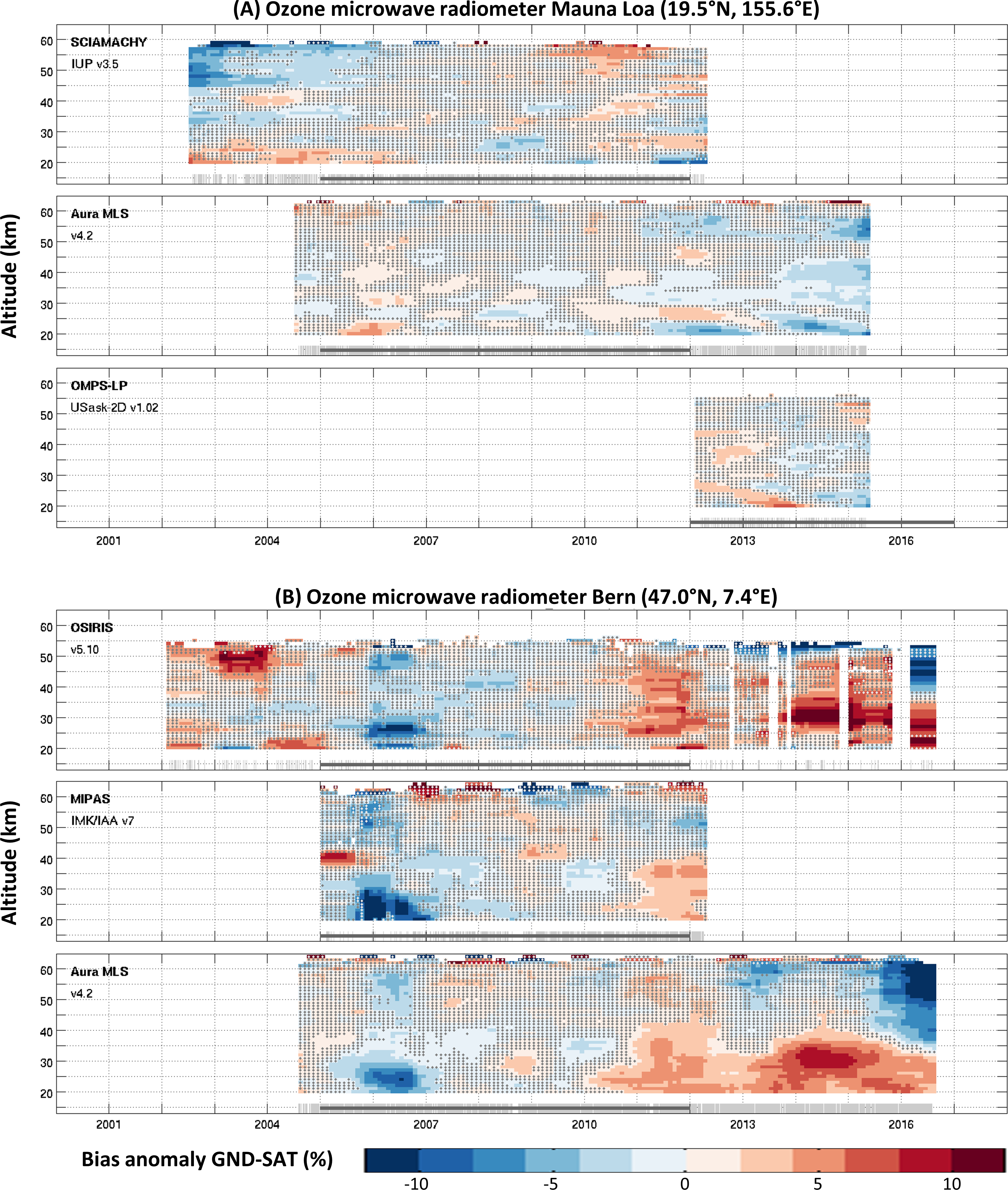	Figure 3.4 | high-res .png As Figure 3.2 but for two microwave radiometer sites. Stippled areas denote non-significant δ values. Comparisons to all six satellite records for both stations are shown in Figures S3.5 and S3.6 in the Supplement. Adapted from Hubert et al. (2019).
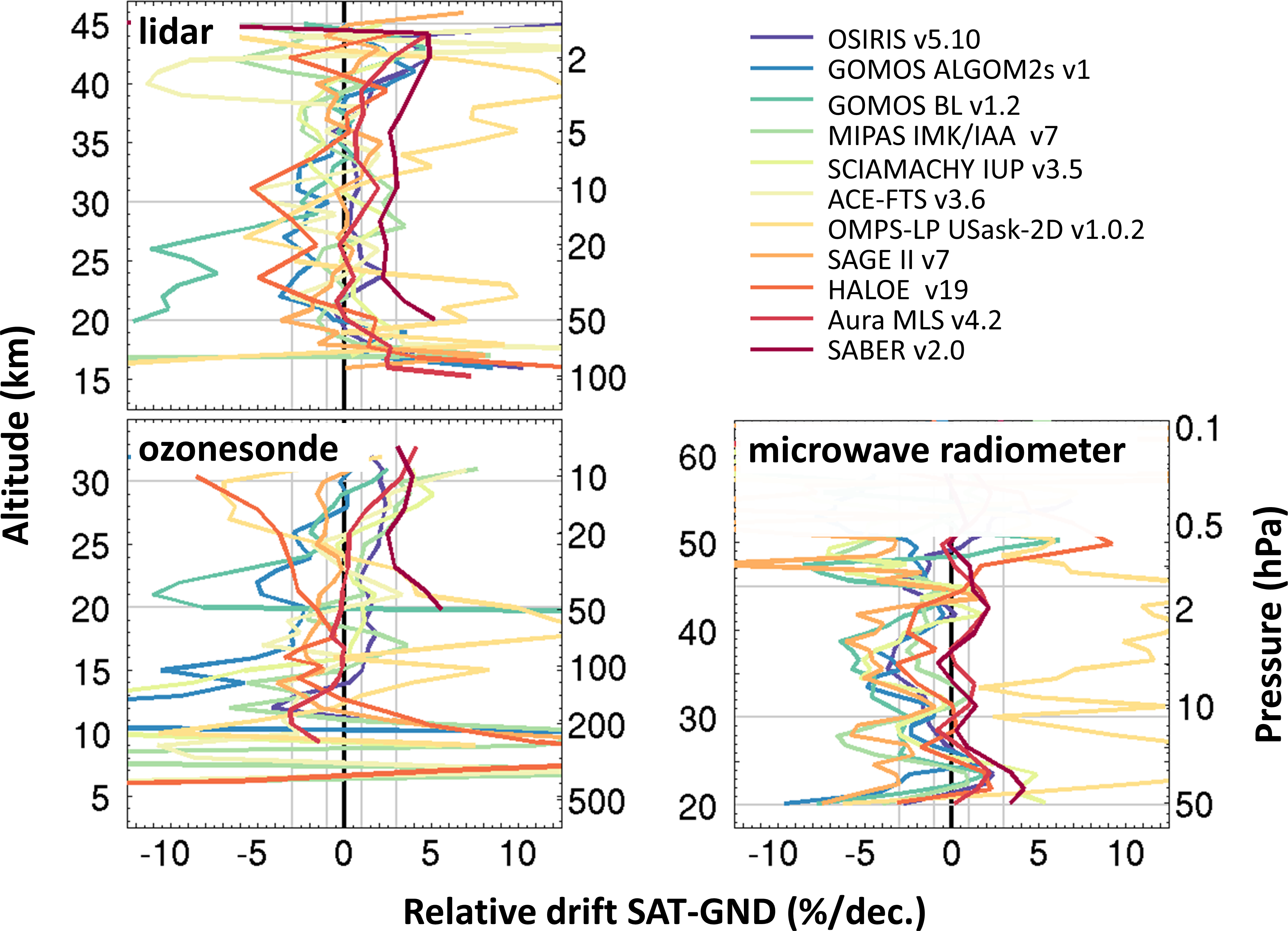	Figure 3.5 | high-res .png Vertical profile of network-averaged satellite drift (Level-2) relative to co-located ground-based measurements by ozonesonde (bottom left), lidar (top left) and microwave radiometer (bottom right). Colours represent different limb/occultation data records (see legend).
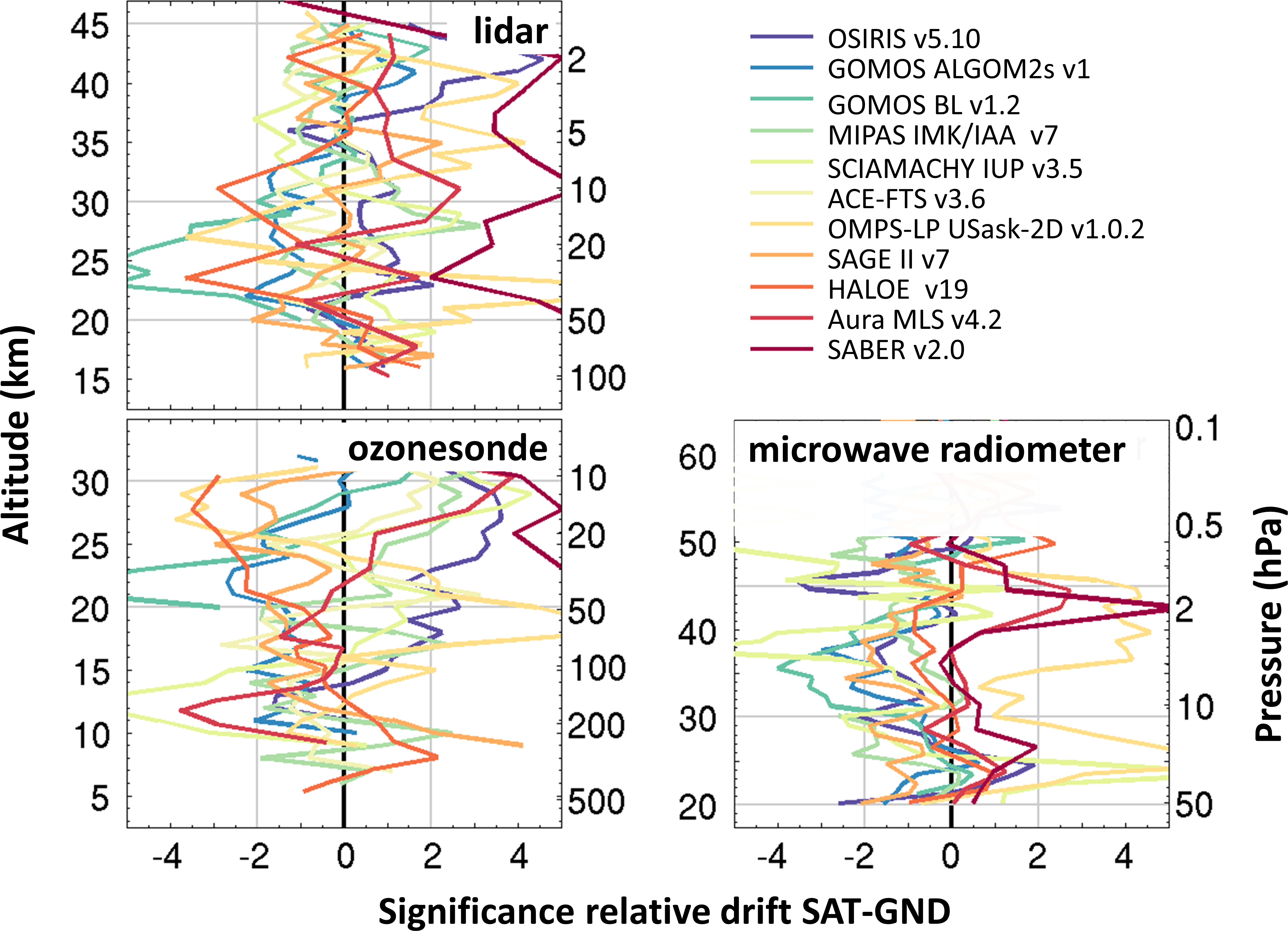	Figure 3.6 | high-res .png As Figure 3.5 but for the significance of the drift estimates. The 2σ detection threshold is indicated by grey vertical lines.
	Figure 3.7 | high-res .png Drift estimates and 95 % confidence interval of monthly zonal mean satellite data relative to the ground-based ozonesonde network. Eight limb/occultation records and the merged SAGE-CCI-OMPS (central panel) are shown. Satellite records contributing to the merged record are indicated with a red asterisk.
	Figure 3.8 | high-res .png Deviations (in %, colour) of deseasonalised anomalies for GOMOS, MIPAS, SCIAMACHY, OSIRIS, ACE-FTS, OMPS, and SAGE II (indicated in the panels) from the median deseasonalised anomalies computed using all data sets. Latitude band is 30°S–40°S. From Sofieva et al. (2017).
	Figure 3.9 | vector .pdf | high-res .png ILT trend proxy fit to 35S–50S monthly zonal mean SBUV MOD (red) and SBUV COH (blue, referred to as “NOAA” in Figure) records over the 2001–2015 time period. The shaded regions indicate the 2-sigma statistical uncertainty estimated from the unexplained variability in the multiple regression analysis. The dotted error bars show the total trend uncertainty when the SBUV MOD 2-sigma merging uncertainty is included. The uncertainties are combined using the root sum of squares of each error term. For comparison, the estimated MOD uncertainty is also added to the SBUV COH error bars. From Frith et al. (2017).
	Figure 3.10 | vector .ps | high-res .png Drift (in % per year) of zonally averaged profile data from SBUV MOD (turquoise) and SBUV COH (red) relative to Aura MLS v4 for 50°S–35°S (left), 20°S–20°N (middle) and 35°N–50°N (right).
	Figure 3.11 | high-res .png Latitude weighted mean 1-sigma errors (%) estimated from the application of SVD for three number density composites (SAGE-MIPAS-OMPS (SMO), SAGE-CCI-OMPS (CCI), and SAGE-OSIRIS-OMPS (SOO)) and the 1-sigma uncertainty in the BASICNDEN composite (dotted black line) derived from these, and for four VMR-based composites (SWOOSH, GOZCARDS, SBUV MOD, and SBUV COH) and the BASICVMR composite (solid black line). Note that number density is on altitude, and VMR on pressure level, so comparing between the VMR and number density data sets is only indicative.
	Figure 3.12 | vector .ps | high-res .png Selected pressure levels in three latitude bands for the four VMR composites and the BASICVMR composite. Each pair of plots show the relative (%) deseasonalised time series bias-shifted to agree with SWOOSH for the July 2005 to December 2013 period (upper half) and anomalies relative to the BASICVMR composite (lower half). The 2-sigma uncertainty on the BASICVMR is shown with grey shading.
	Figure 3.13 | vector .ps | high-res .png As for Figure 3.12 but for the number density composites and BASICNDEN derived from these.
	Figure 3.14 | high-res .png Two levels from Figures 3.12 and 3.13 overlaying the VMR and number density time series for comparative purposes. Each pair of plots show the relative (%) change compared to the July 2005 – December 2012 mean (a & c) and the change relative to BASICVMR (b & d). Note that while number density and VMR time series shown correspond to approximately the same region in the atmosphere, they are not exact and should be considered only indicative.
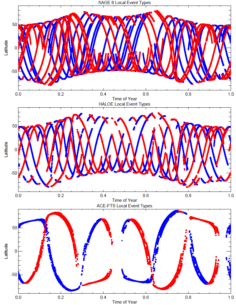	Figure 3.15 | high-res .png Latitude and time of year of all events for SAGE II, HALOE, and ACE-FTS separated by local event type (blue for sunrise and red for sunset) plotted every 3 years (to reduce clutter) illustrating the drifting sampling patterns over time. Sampling patterns can systematically shift several weeks over a few years for instruments like SAGE II (in its later years) or HALOE (continuously) while ACE-FTS is essentially constant. Time of year is expressed as the modulus of the year fraction.
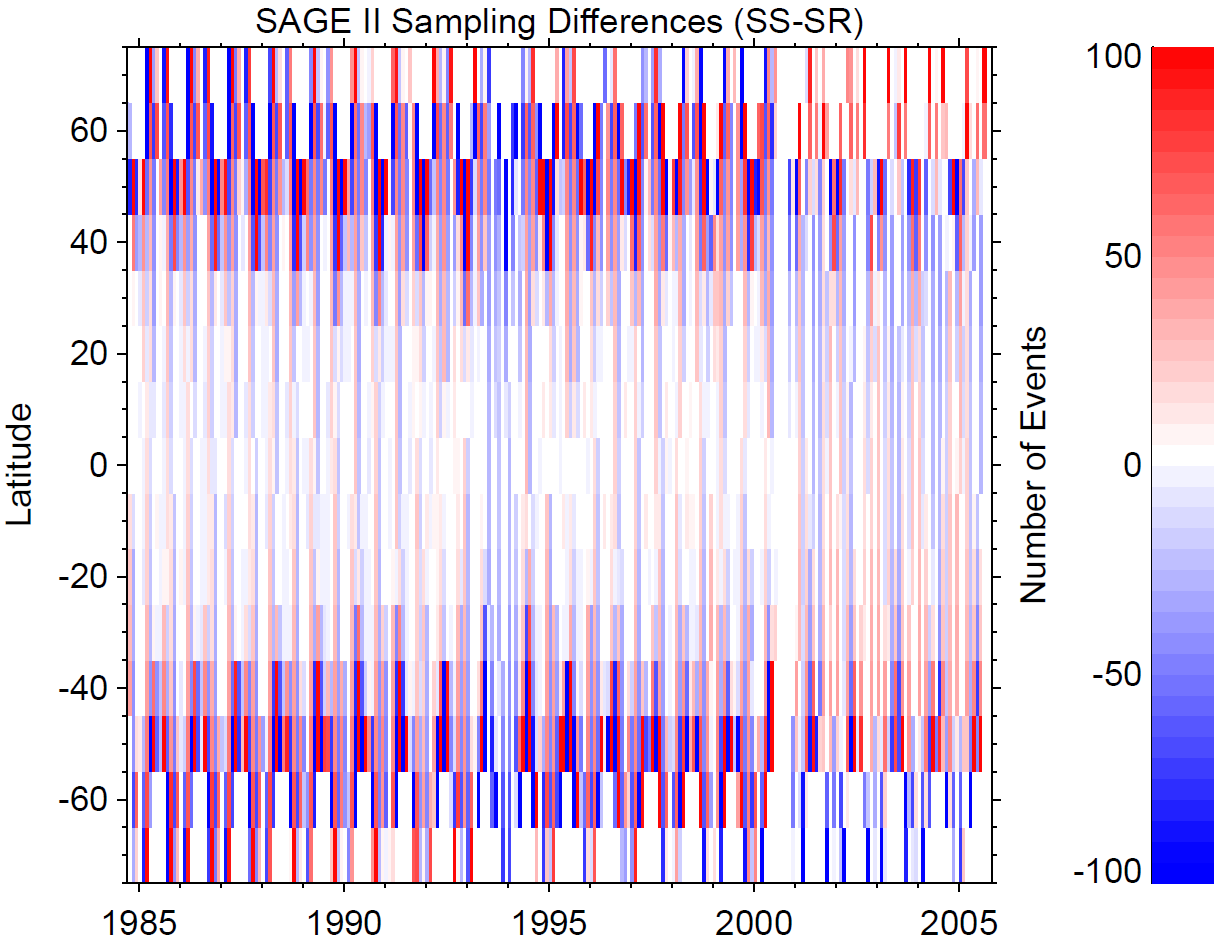	Figure 3.16 | high-res .png The difference in the total number of sunset (SS) and sunrise (SR) events in each month and 10 degree latitude bin from SAGE II. In addition to the rapid oscillation between SR and SS dominated months, instrument anomalies resulted in large periods and locations of SR/SS dominated sampling (bottom panel of Figure 8 of Damadeo et al., 2018).
	Figure 3.17 | vector .ps | high-res .png Long-term trends derived from both the MZM and the STS regressions during the potential recovery period. Results are also shown when using the STS regression results to create a diurnally corrected (DCorr) and a diurnally & seasonally corrected (DSCorr) data set for use with the MZM regression. The diurnal correction has the greatest influence on the upper stratosphere while the seasonal correction has the greatest influence at higher latitudes. Stippling denotes areas where the trend results are not significant at the 2σ level. Contour lines are plotted at 2 % intervals. (Figure 11 from Damadeo et al., 2018).
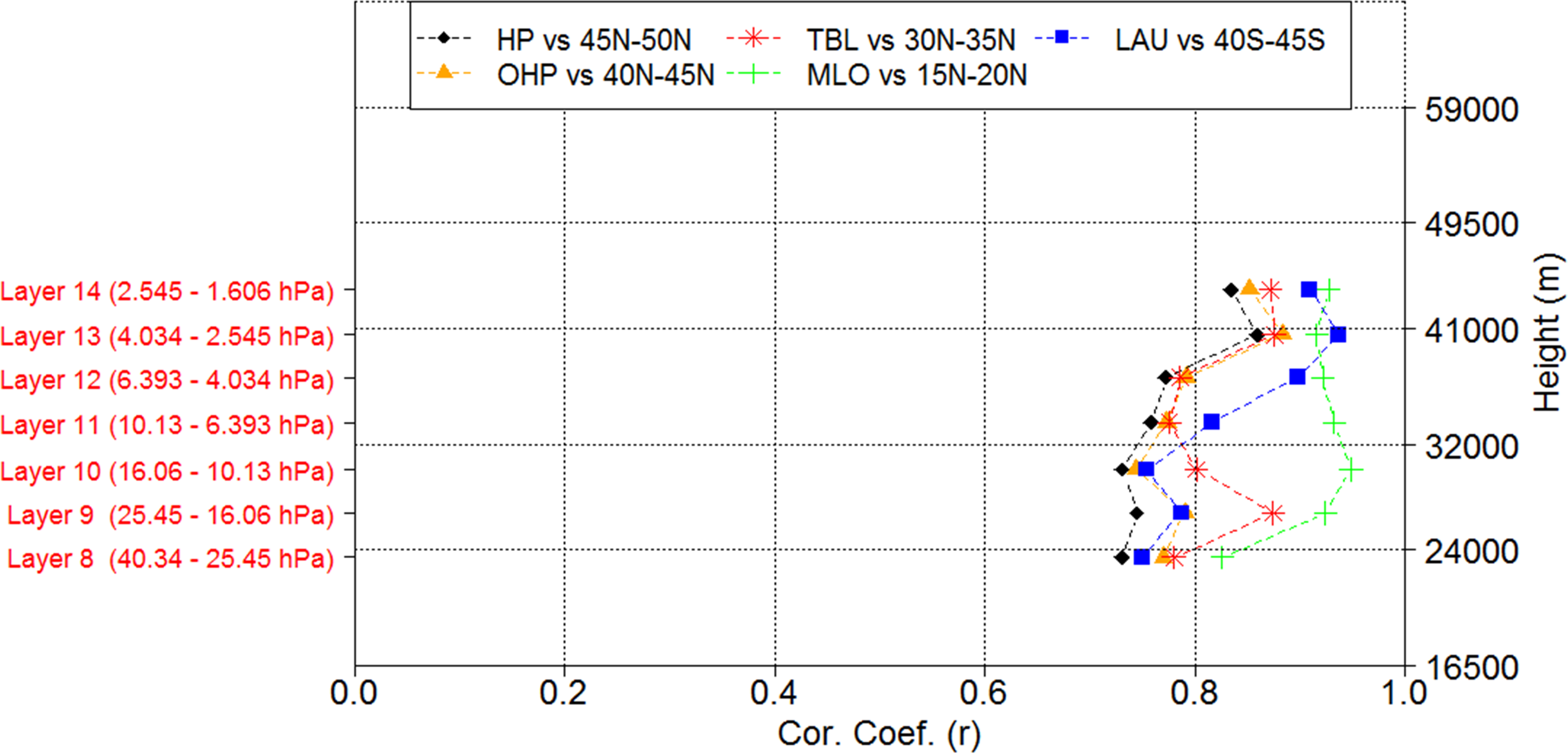	Figure 3.18 | high-res .png Correlation between monthly mean SBUV overpass data at five lidar stations versus the corresponding 5° monthly zonal mean SBUV data of each site. (Figure 2a from Zerefos et al., 2018).
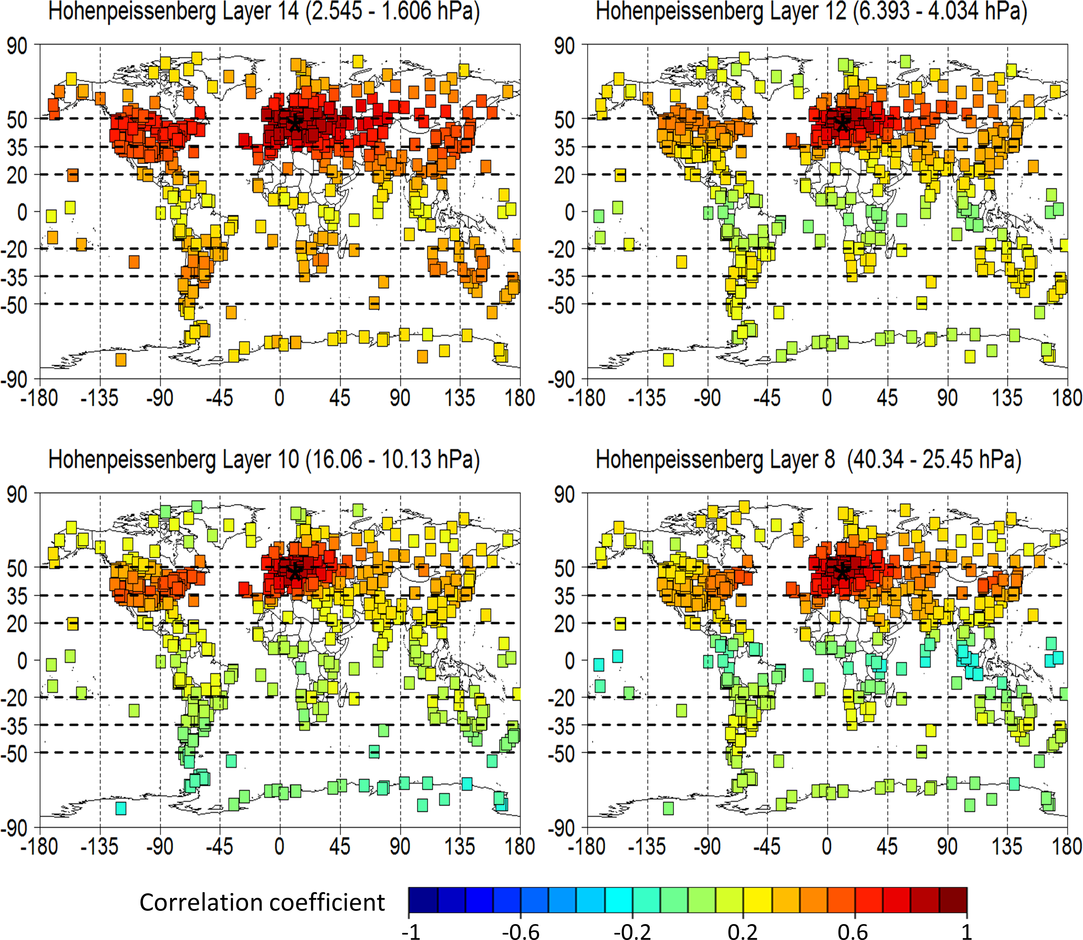	Figure 3.19 | high-res .png Correlation between the time series, previously deseasonalised and known variability removed, of layered ozone monthly SBUV MOD overpasses at the Hohenpeissenberg station and the SBUV MOD overpasses at various other locations around the globe. Four layers are shown in the panels. The black star indicates the location of Hohenpeissenberg.

Chapter 4

	Figure 4.1 | vector .eps | high-res .png The leading two EESC EOF terms derived from multiple mean age-of-air EESC time series proxies.
	Figure 4.2 | vector .pdf | high-res .png Derived ozone trends in percent per decade from the 15 different regressions applied to the same SBUV MOD data set between 35°N–50°N (top) and 50°S–35°S (bottom). In each plot, the dashed/solid lines represent trend values before/after 1997 at each of the 9 pressure levels.
	Figure 4.3 | vector .eps | high-res .png Standard errors between 5°S–5°N at 30 km used for the weighted regression applied to the merged SAGE-OSIRIS-OMPS ozone data set both before and after the heteroscedasticity correction. Note how the errors/weights before the correction drop/rise dramatically once OSIRIS (added in 2001) and OMPS (added in 2012) are added as a result of increased sampling of the instruments.
	Figure 4.4 | vector .eps | high-res .png Rolling (running average) standard deviation of the residuals of the weighted regression between 5°S–5°N at 30 km both with and without the heteroscedasticity correction. In addition to generally reducing the spread of the residuals of the fit, the heteroscedasticity correction also makes the rolling standard deviation more uniform throughout the data. Prior to the correction, the rolling standard deviation (not the standard error) increased when moving from SAGE II data to OSIRIS and later OMPS data.
	Figure 4.5 | vector .eps | high-res .png Impact on potential recovery trends depending on the cutoff time of the regression for different solar proxies when applied to the SAGE-OSIRIS-OMPS data set centred at 40°S at 40 km. The impact on resulting trends of ignoring the solar proxy is evident for all but the longest data records while it is also apparent that the f10.7 and Mg II proxies have negligibly different impacts relative to each other.
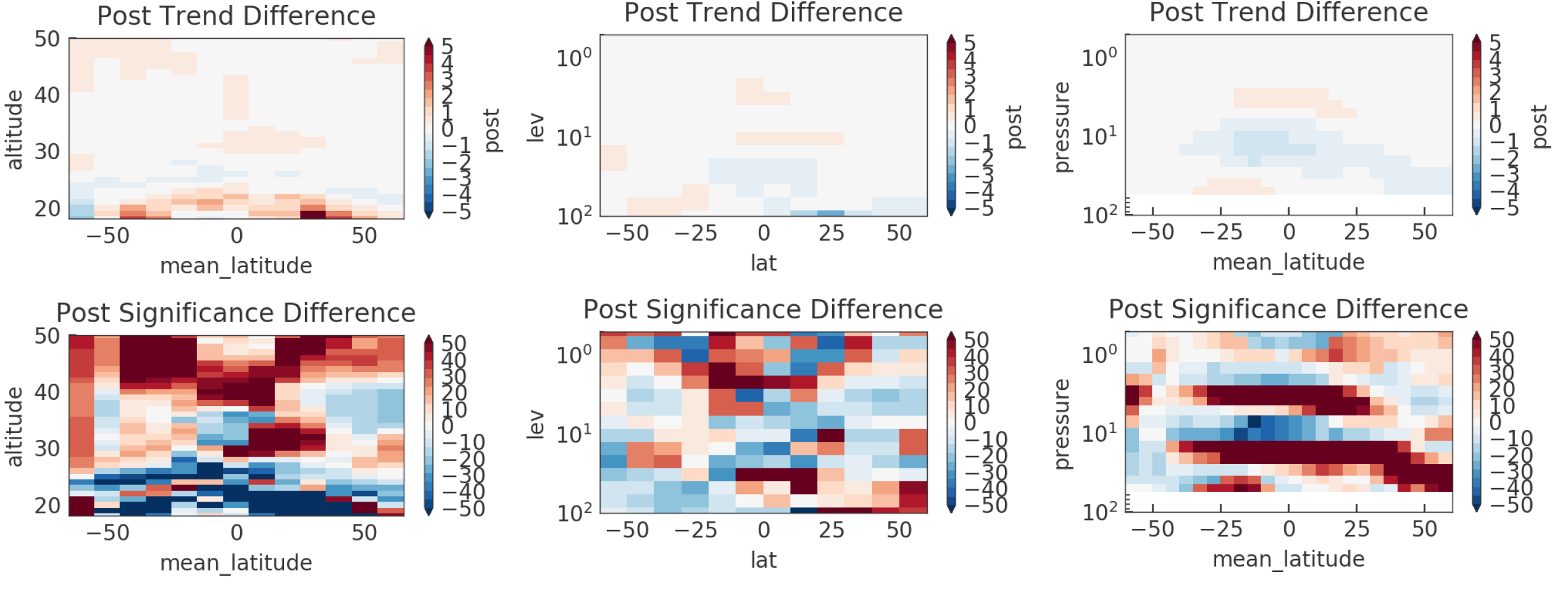	Figure 4.6 | high-res .png Influence on the “Post-2000” trends (top row) and significances (bottom row) when adding the GISS aerosol proxy for the SAGE-OSIRIS-OMPS (left column), GOZCARDS (middle), and SBUV COH (right) data sets.
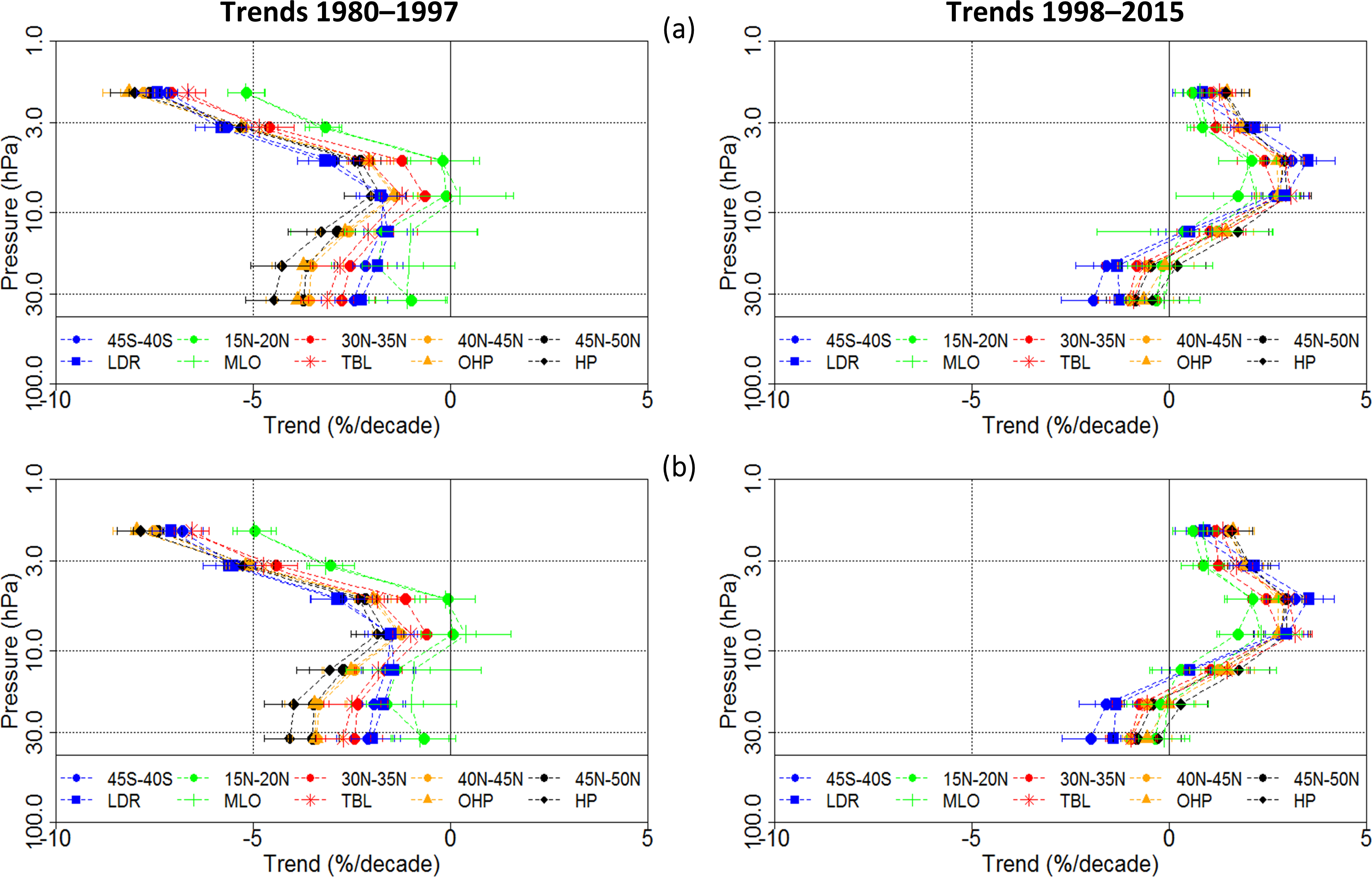	Figure 4.7 | high-res .png Adapted from Figure 7 of Zerefos et al. (2018) showing trends in the vertical distribution of ozone for the pre-1998 and post-1998 period, using (a) two linear trend terms (PWLT method) and volcanic effects and (b) the PWLT method including all proxies. The results are based on SBUV zonal means and SBUV overpasses over five lidar stations (LDR=Lauder, MLO=Mauna Loa Observatory, TBL=Table Mountain, OHP=Haute Provence, HP=Hohenpeissenberg).
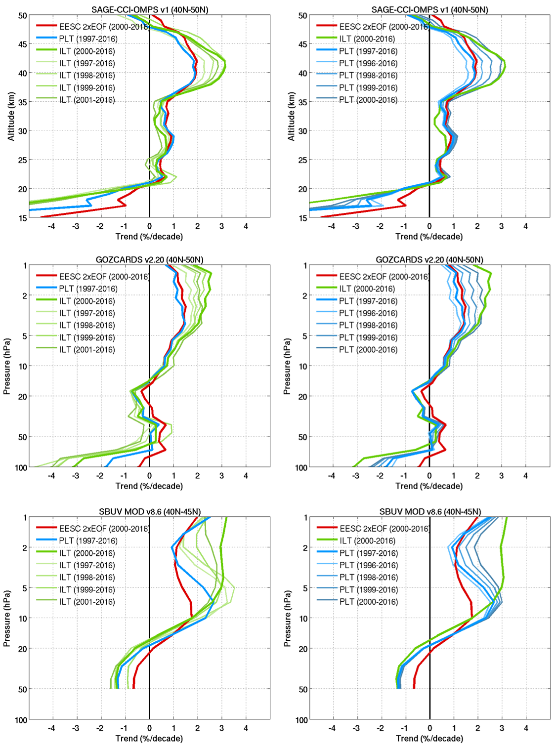	Figure 4.8 | high-res .png Effect of time period start and end points on ozone trends in the past two decades obtained by regressions with PWLT and ILT.
	Figure 4.9 | vector .eps | high-res .png Derived trends in ozone in percent per decade for the SAGE II-OSIRIS-OMPS data set (using the sampling bias adjusted SAGE II data from Damadeo et al., 2018) for both the pre-1997 (start of 1985 to end of 1996, top row) and post-2000 (start of 2000 to end of 2016, bottom row) time periods. Results are shown for each of the three trend proxies: The PWLT (left), ILT (middle), and EESC EOFs (right) proxies. Stippling denotes results that are not statistically significant at the 2-sigma level.
	Figure 4.10 | vector .eps | high-res .png As Figure 4.9 but for the GOZCARDS data set.
	Figure 4.11 | vector .eps | high-res .png As Figure 4.9 but for the SBUV MOD data set.

Chapter 5

	Figure 5.1 | vector .eps | high-res .png Derived trends in satellite ozone in percent per decade for the pre-1997 period (Jan 1985 – Dec 1996) for each of the satellite data sets, using the ILT trend proxy in a regression analysis. Grey stippling denotes results that are not significant at the 2-sigma level. Data are presented on their natural latitudinal grid and vertical coordinate. For comparison, the mean of trends derived from CCMI participating models is included in the upper left panel. Results for other trend proxies can be found in the Supplement.
	Figure 5.2 | vector .eps | high-res .png Derived trends in satellite ozone in percent per decade for the post-2000 period (Jan 2000 – Dec 2016) for each of the satellite data sets, using the ILT trend proxy in a regression analysis. Grey stippling denotes results that are not significant at the 2-sigma level. Data are presented on their natural latitudinal grid and vertical coordinate. For comparison, the mean of trends derived from CCMI participating models is included in the upper left panel. Results for other trend proxies can be found in the Supplement.
	Figure 5.3 | vector .pdf | high-res .png Impact of sampling bias correction on ozone trends derived from the SAGE-ORIRIS-OMPS data set. Grey stippling denotes where the trends derived from either version of data (i.e., sampling-corrected or not) were not significant at the 2-sigmal level.
	Figure 5.4 | vector .pdf | high-res .png The evolution of ozone changes as annual mean anomalies at the 2 hPa/42 km (left panel) and 10 hPa/31 km (right panel) levels. Three different latitude bands are shown. Satellite data are based on zonal means, and ground-based stations are averaged over the latitude bands. The grey “envelope” gives the CCMI-1 model results, based on the models’ 10th and 90th percentile. The model mean and the median are also plotted together with the ±2 standard deviation range of the models. All anomalies are calculated over the base period 1998–2008, and the CCMI-1 models are shown as 1-2-1 year filtered averages (see text).
	Figure 5.5 | vector .pdf | high-res .png Same as Figure 5.4 but for the 20 hPa/26 km (left panel) and 70 hPa/19 km (right panel) levels.
	Figure 5.6 | vector .pdf | high-res .png Ozone trends with 2-sigma uncertainties for the pre-1997 (top) and post-2000 (bottom) period from the ILT regression for latitude bands 60°S–35°S (left), 20°S–20°N (centre), and 35°N–60°N. Coloured lines are the trend estimates from individual merged data sets on their original vertical grid.
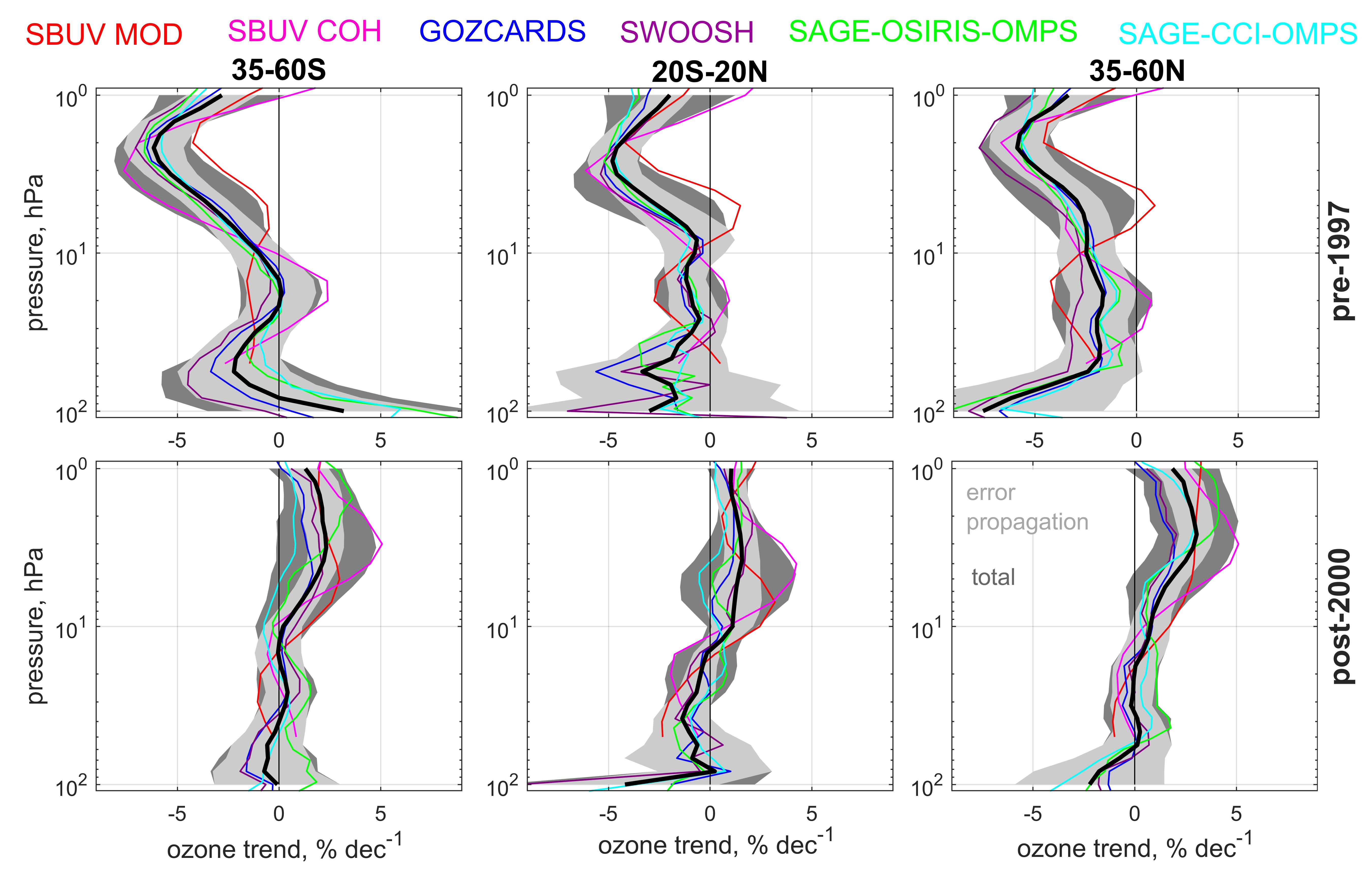	Figure 5.7 | high-res .jpg Combining pre-1997 (top) and post-2000 (bottom) trend estimates and uncertainties (2-sigma) by Equation (5.1) from six limb profile data sets. Black solid line indicates the mean trend. The uncertainty component corresponding to error propagation (1st term in Equation (5.1)) is shown by light grey shading, while the total uncertainty is indicated by dark grey shading.
	Figure 5.8 | vector .pdf | high-res .png Combined trends of six limb and nadir data records (thick black lines) with 2-sigma uncertainties (thin coloured lines) for the pre-1997 period (top) and the post-2000 period (bottom) from the ILT regression for latitude bands 60°S–35°S (left), 20°S–20°N (centre), and 35°N–60°N. Green lines denote results from the LOTUS method (Equation 5.1), blue lines denote results from the method of Steinbrecht et al. (2017; Equation 5.5) with neff = 2 for pre-1997 and neff = 3 for post-2000 trends, and red lines denote the results from the J-distribution method (Equation 5.4).
	Figure 5.9 | vector .pdf | high-res .png Ozone trends for the pre-1997 and post-2000 periods from the ground-based stations, averaged over the available latitude bands. Upper panel shows 35°N–60°N, middle panel shows 20°S–20°N, and lower panel shows 60°S–35°S.
	Figure 5.10 | vector .pdf | high-res .png Ozone profile trends from different groundbased data records for the pre-1997 (left) and post-2000 periods (right) at Hawaii, USA (19.5–19.7°N, 155.1–155.6°W; top row) and at Lauder, New Zealand (45.0°S, 169.7°W; bottom row). Error bars represent the 95 % confidence interval. The black line represents the multi-model mean for the latitude band 15°N–25°N and 50°S–40°S, respectively.
	Figure 5.11 | vector .pdf | high-res .png Ozone trends for the pre-1997 and post-2000 periods from the CCMI REF-C2 models’ simulation and broadband satellite data sets, averaged over the available latitude bands: 35°N–60°N (upper panel), 20°S–20°N (middle panel), and 60°S–35°S (lower panel).
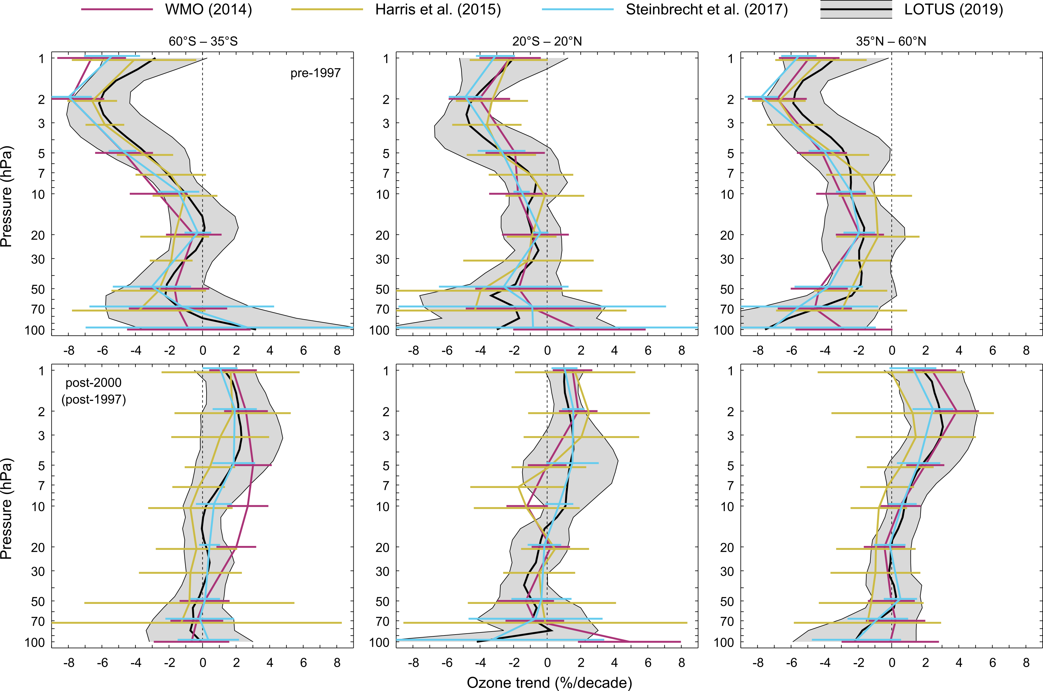	Figure 5.12 | high-res .png Overview of ozone profile trends from past and recent assessments: LOTUS (this work), WMO (2014), Harris et al. (2015), and Steinbrecht et al. (2017) are shown in black, red, orange, and blue respectively. Top row shows trends before the turnaround of ODSs and bottom row since the turnaround (analysis time period differs by assessment). Shaded area and error bars represent the 95% confidence interval for the combined trend. Coloured profiles are slightly offset on the vertical axis for display purposes.
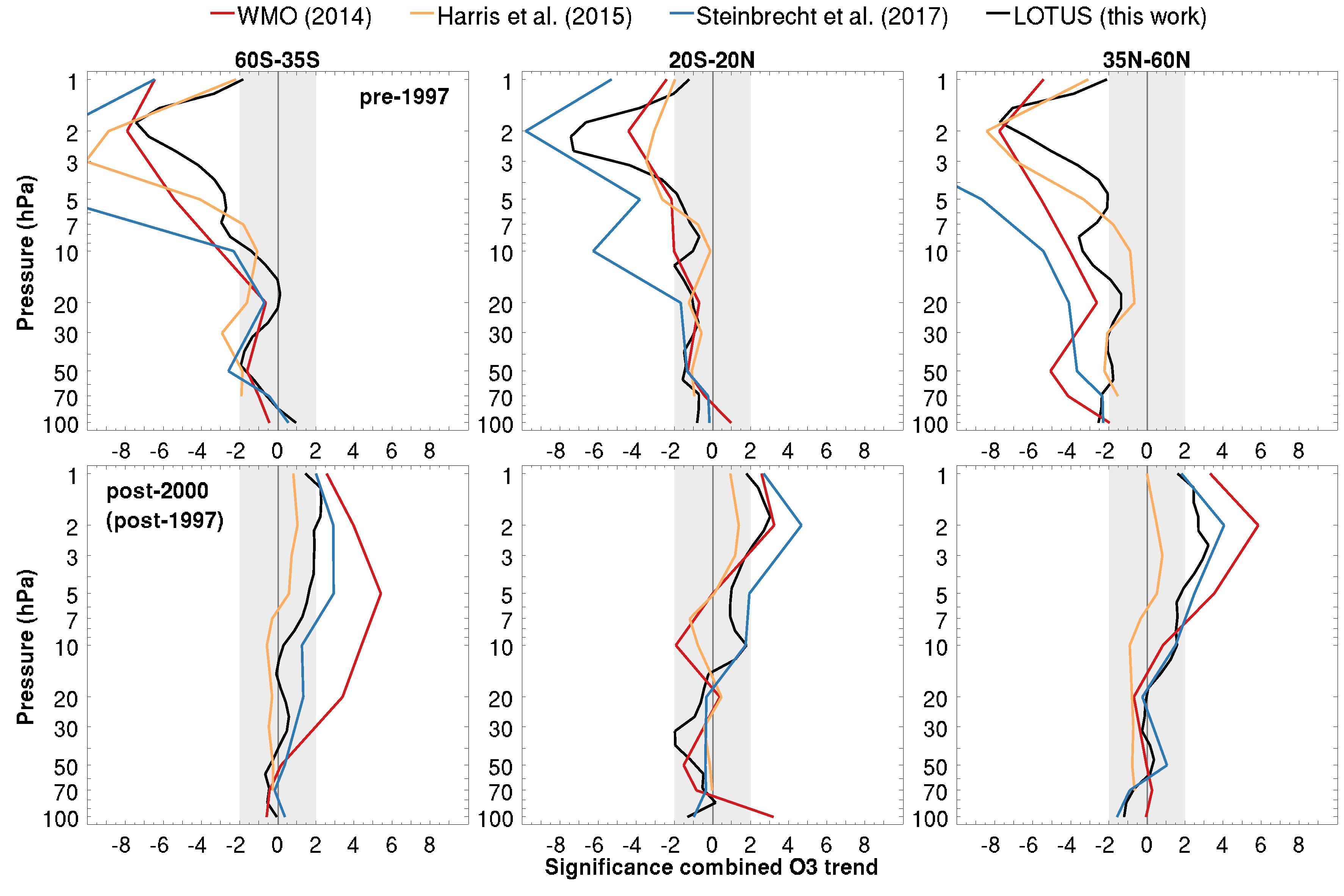	Figure 5.13 | high-res .png As in Figure 5.12 but for the significance of ozone profile trends from past and recent assessments.
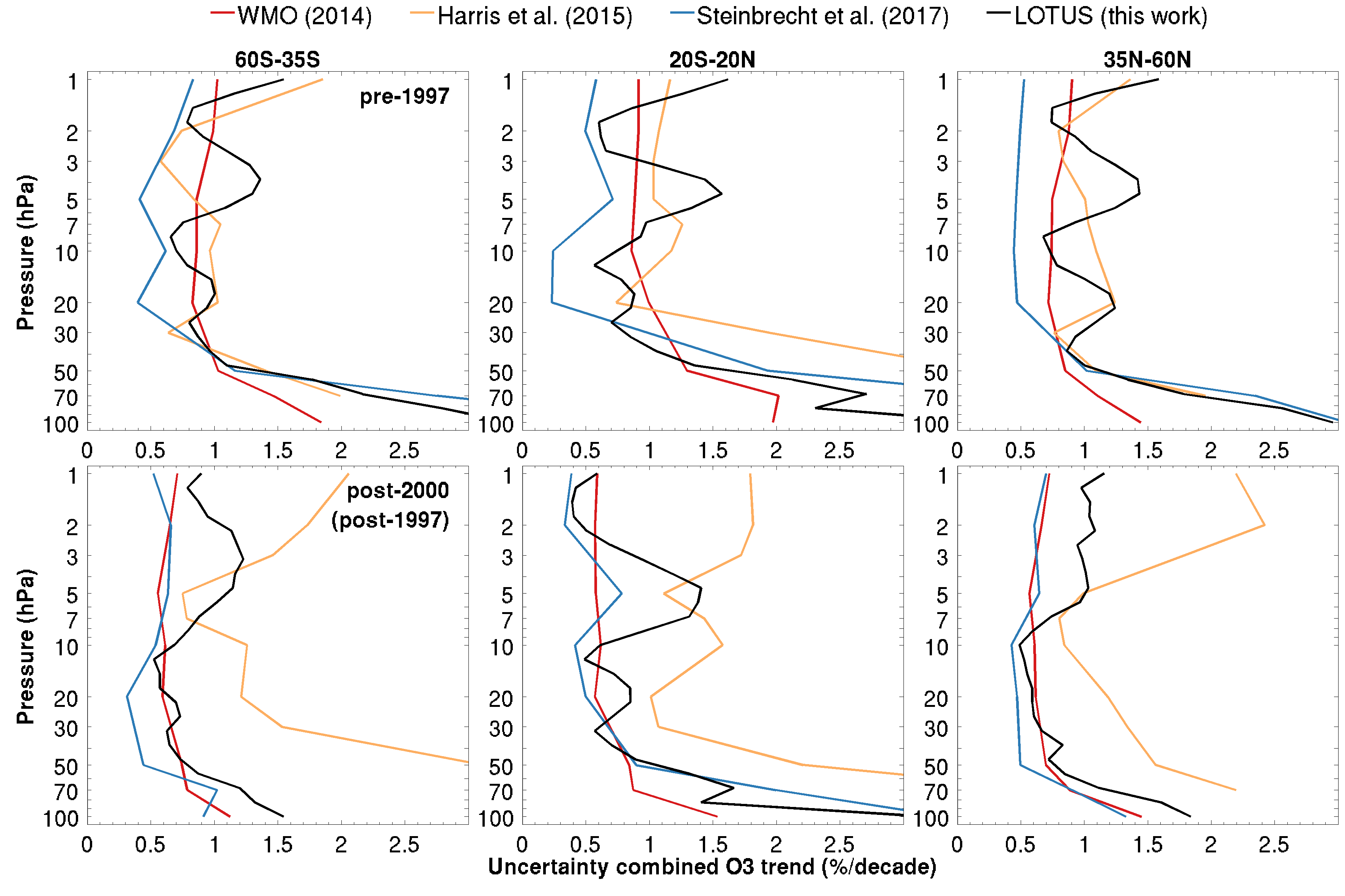	Figure 5.14 | high-res .png As in Figure 5.12 but for the uncertainty (1-sigma) of ozone profile trends from past and recent assessments.

Supplement

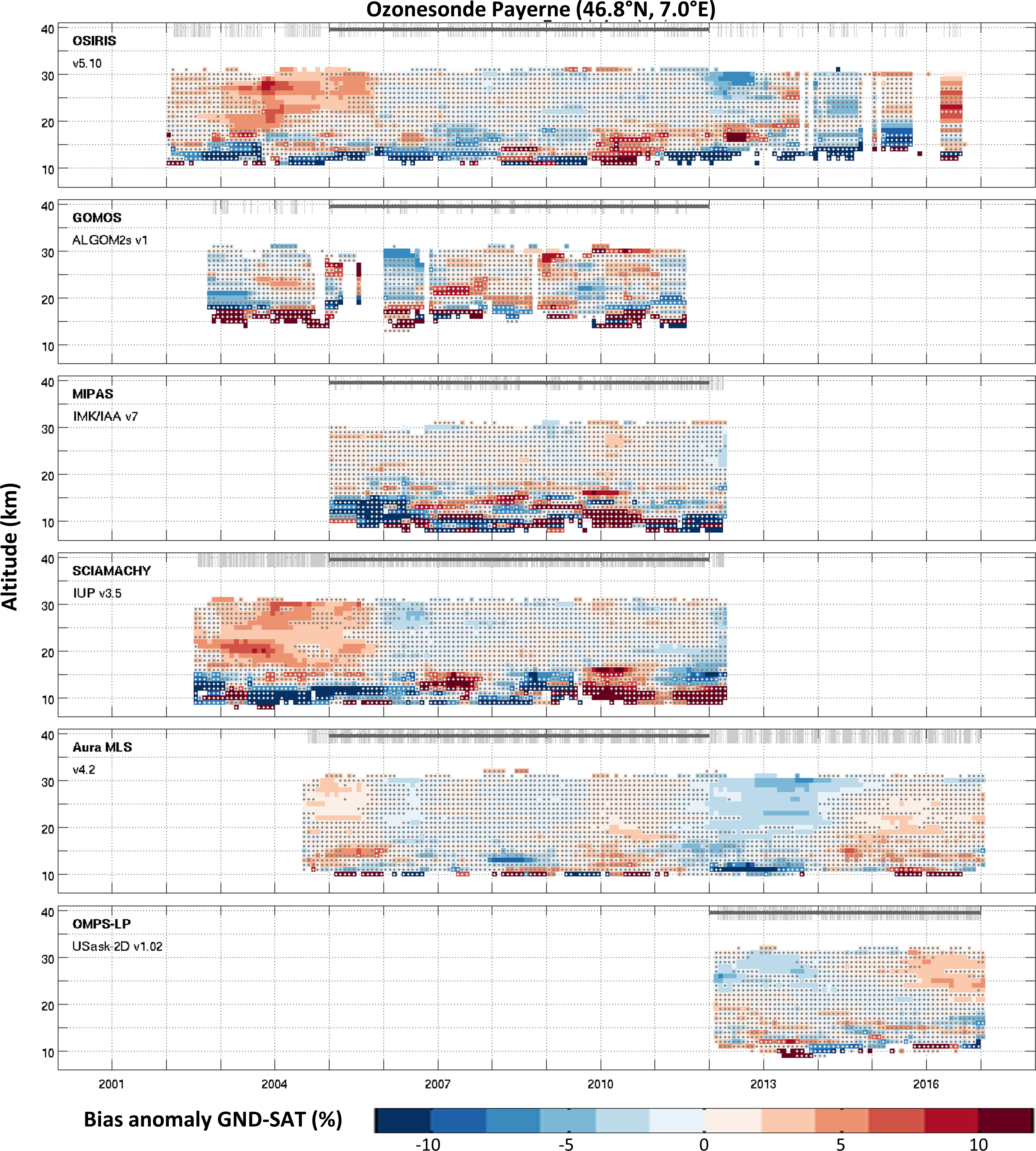	Figure S3.1 | high-res .png Smoothed anomaly time series (δ, see Equation 3.1) of the relative difference of Payerne ozonesonde and six satellite ozone profile data records (top to bottom). Red values indicate regions in which sonde measurements are biased more positive (or less negative) compared to satellite than their median value during the reference period. Stippled areas denote δ values that are not statistically different from zero at the 2-sigma level. A running average with a 12-month window was used to smooth the time series. Thin grey vertical lines show the sampling of the co-located profile data records; the grey horizontal lines indicate the reference period for each comparison. A selection of these panels was shown in Figure 3.2. Adapted from Hubert et al. (2019).
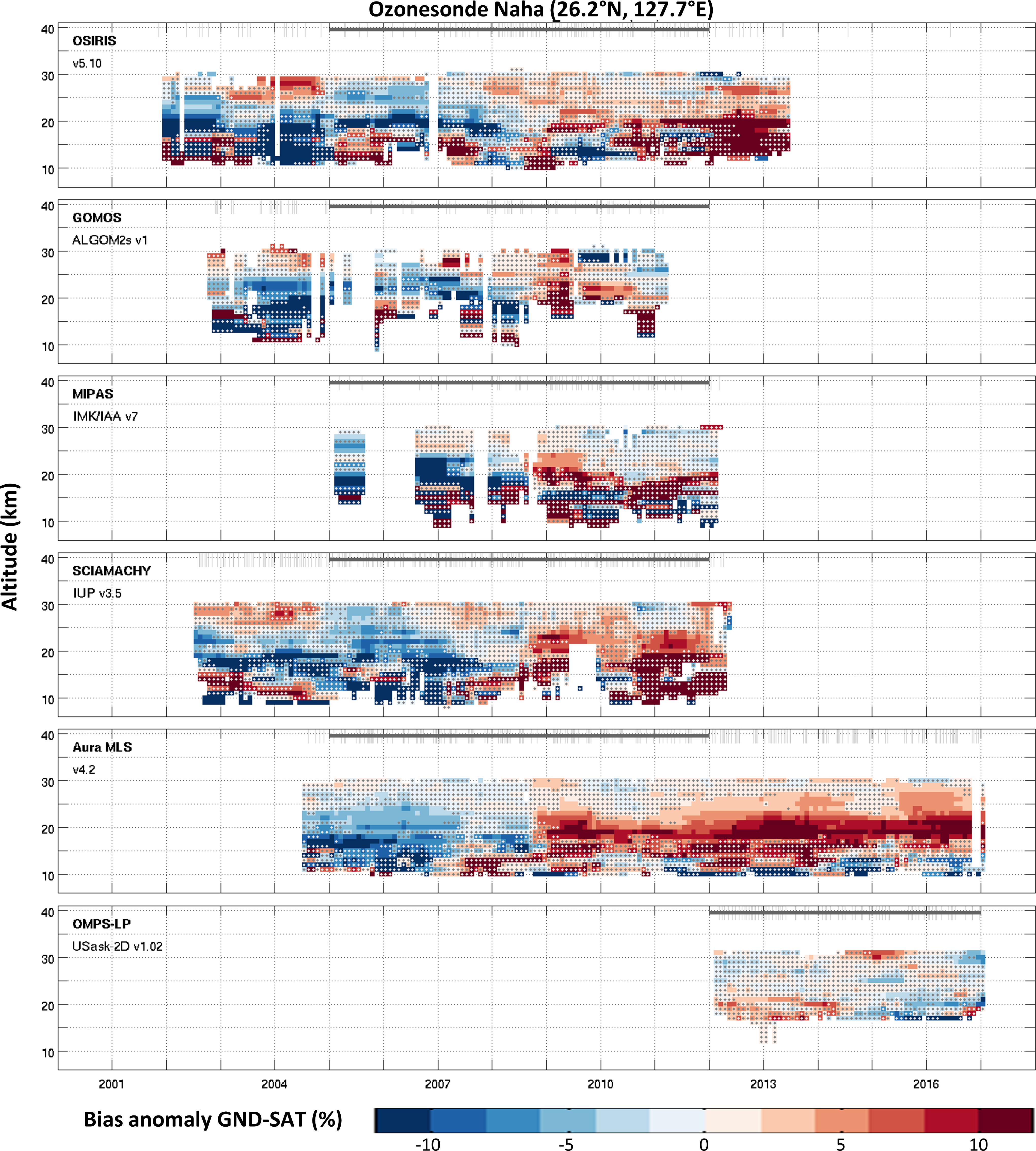	Figure S3.2 | high-res .png As Figure S3.1, but for the Naha ozonesonde. Stippled areas denote non-significant δ values. A selection of these panels was shown in Figure 3.2. Adapted from Hubert et al. (2019).
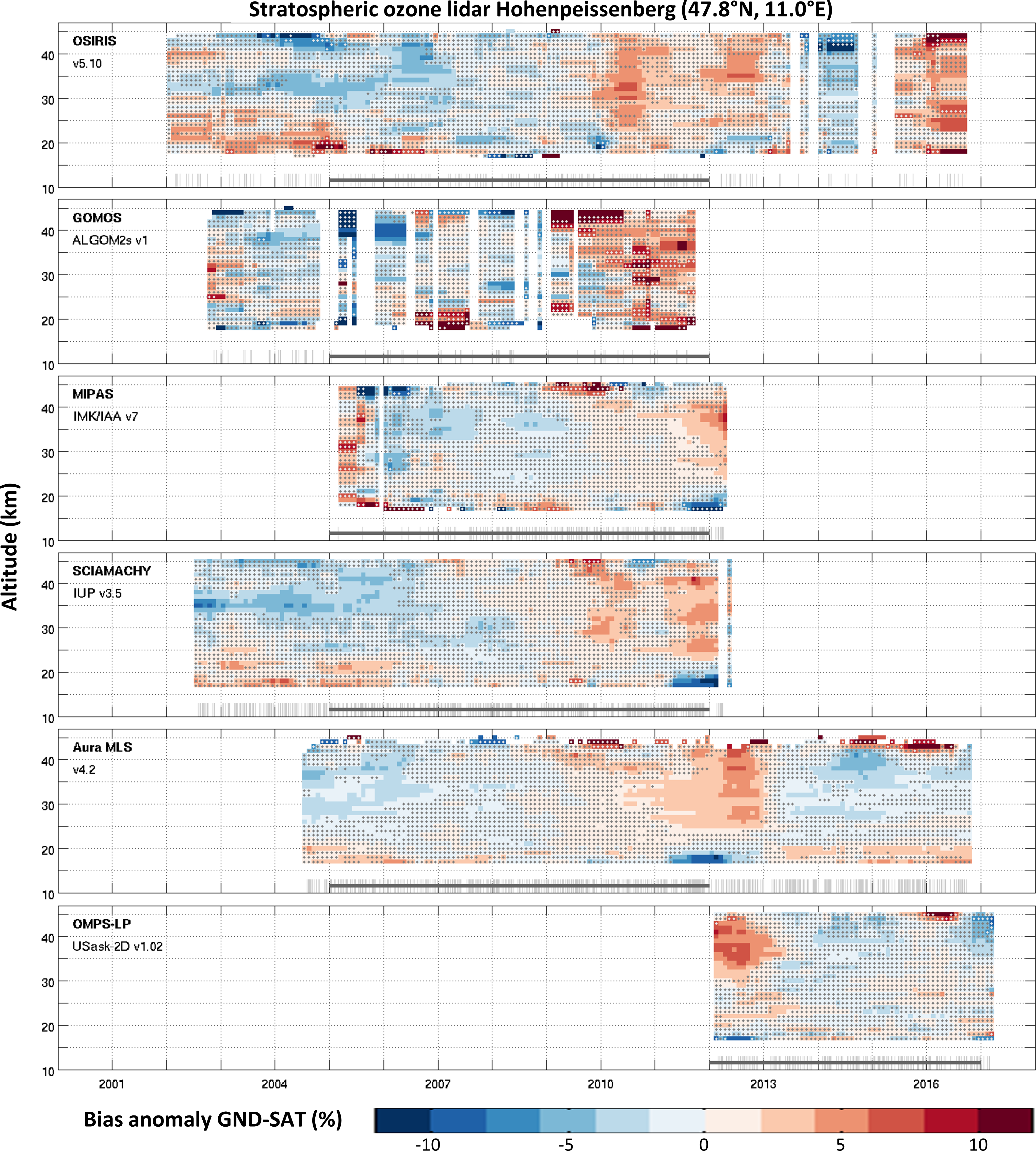	Figure S3.3 | high-res .png As Figure S3.1, but for the Hohenpeissenberg lidar. Stippled areas denote non-significant δ values. A selection of these panels was shown in Figure 3.3. Adapted from Hubert et al. (2019).
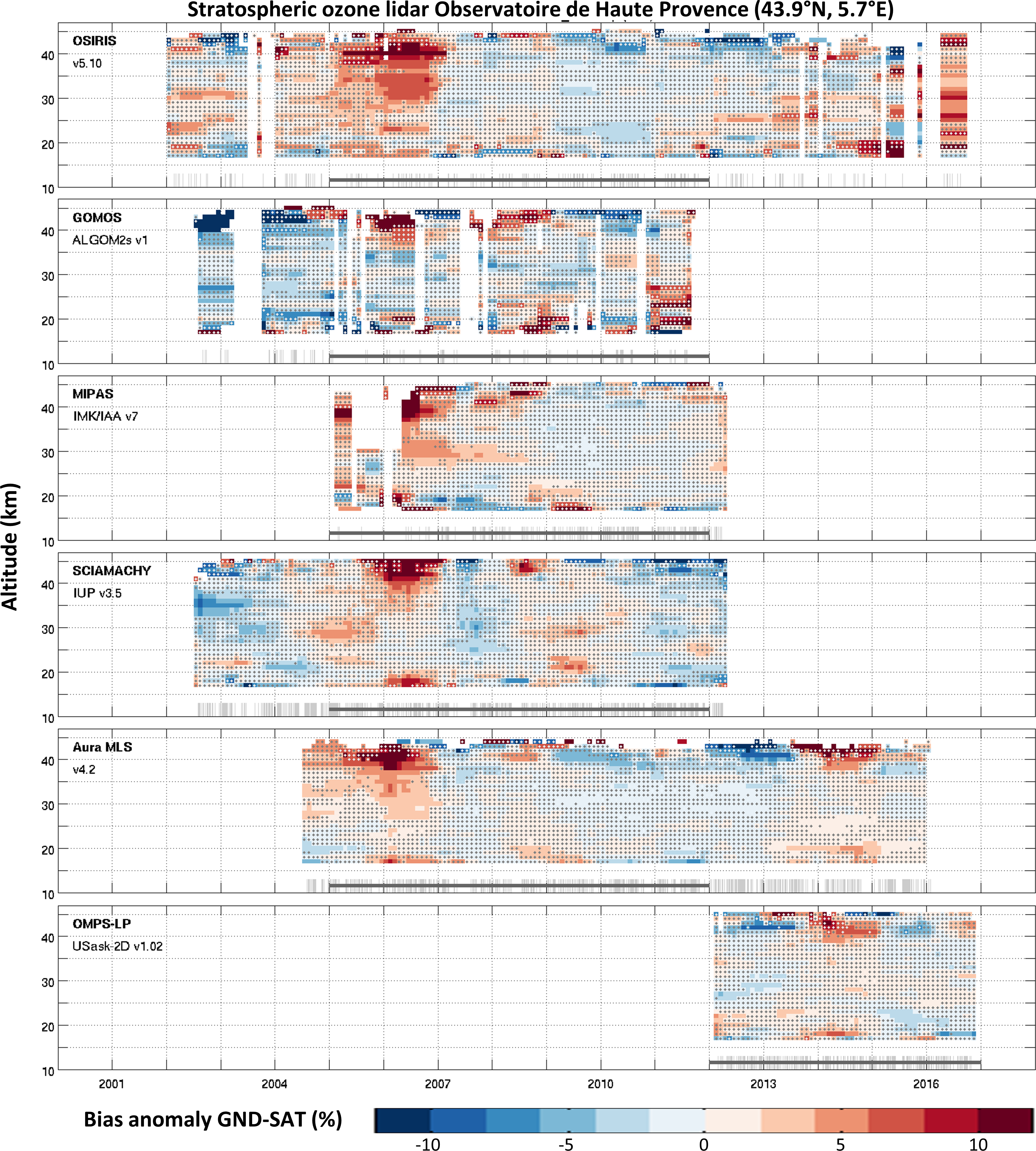	Figure S3.4 | high-res .png As Figure S3.1, but for the OHP lidar. Stippled areas denote non-significant δ values. A selection of these panels was shown in Figure 3.3. Adapted from Hubert et al. (2019).
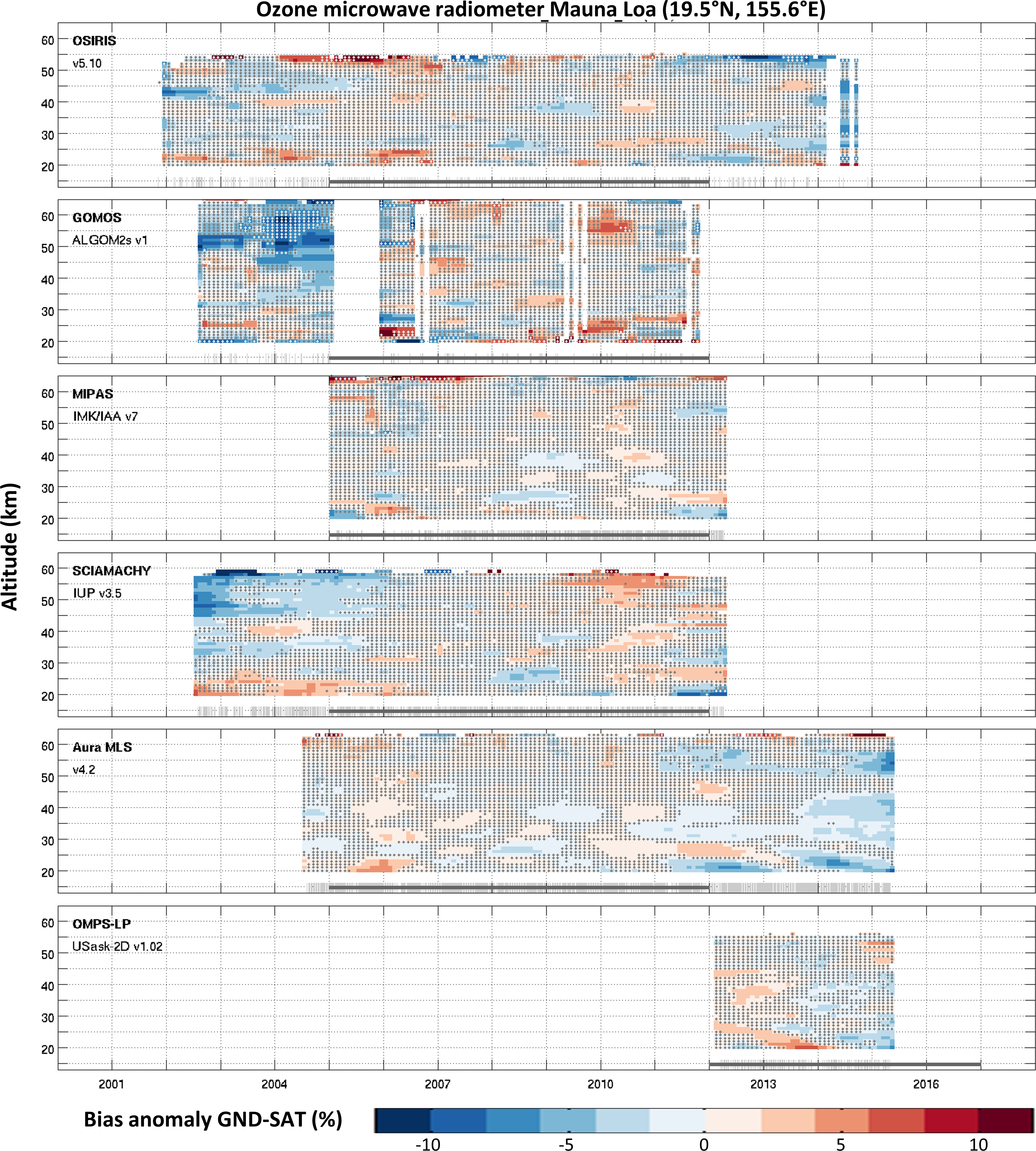	Figure S3.5 | high-res .png As Figure S3.1, but for the MLO radiometer. Stippled areas denote non-significant δ values. A selection of these panels was shown in Figure 3.4. Adapted from Hubert et al. (2019).
	Figure S3.6 | high-res .png As Figure S3.1, but for the Bern radiometer. Stippled areas denote non-significant δ values. A selection of these panels was shown in Figure 3.4. Adapted from Hubert et al. (2019).
	Figure S3.7 | high-res .png Deviations (in %, color) of SCIAMACHY deseasonalised anomalies from the median deseasonalised Anomalies of SAGE II, GOMOS, MIPAS, SCIAMACHY, OSIRIS, ACE-FTS and OMPS. 10° latitude bands are indicated by their centres in the Panels. The dashed line indicates the early part of the mission during which significant deviations from the median deseasonalised Anomalies are observed. From Sofieva et al. (2017).
	Figure S3.8 | high-res .png As Figure S3.7 but for the OMPS-LP deseasonalised anomalies. From Sofieva et al. (2017).
	Figure S4.1 | vector .eps | high-res .png VMR-based profiles of ozone change (%) using DLM analysis for the three broad latitude bands (60°S–35°S, 20°S–20°N, and 35°N–60°N) and two time periods (Jan 1985 to Dec 1999 and Jan 2000 and Dec 2015). Error bars are 2-sigma.
	Figure S4.2 | vector .eps | high-res .png Number density-based profiles of ozone change (%) using DLM analysis for the three broad latitude bands (60°S–35°S, 20°S–20°N, and 35°N–60°N) and two time periods (Jan 1985 to Dec 1999 and Jan 2000 and Dec 2015). Error bars are 2-sigma.
	Figure S4.3 | vector .eps | high-res .png VMR-based and number density profiles of change in ozone (%) from DLM analysis for the three Broad latitude bands (60°S–35°S, 20°S–20°N, and 35°N–60°N) and two time periods (Jan 1985 to Dec 1999 and Jan 2000 and Dec 2015). error bars are 2-sigma. Number density on altitude profiles are approximately scaled to pressure profiles with 100 hPa ~16 km and 1 HPa ~48 km.
	Figure S4.4 | vector .eps | high-res .png VMR-based profiles for change in ozone (scaled to % per decade) from DLM analysis, rescaled From Figure S4-3 for the three broad latitude bands (60°S–35°S, 20°S–20°N, and 35°N–60°N) and two time periods (Jan 1985 to Dec 1999 And Jan 2000 and Dec 2015/2016). Error bars are 2-sigma.
	Figure S5.1 | vector .eps | high-res .png Derived trends in ozone in percent per decade for the pre-1997 period (Jan 1985 - Dec 1996) for each of the satellite data sets, using the PWLT trend proxy in a regression analysis. Grey stippling denotes results that are not significant at the 2-sigma level. Data are presented on their natural latitudinal grid and vertical coordinate.
	Figure S5.2 | vector .eps | high-res .png Derived trends in ozone in percent per decade for the post-2000 period (Jan 2000 - Dec 2016) for each of the satellite data sets, using the PWLT trend proxy in a regression analysis. Grey stippling denotes results that are not significant at the 2-sigma level. Data are presented on their natural latitudinal grid and vertical coordinate.
	Figure S5.3 | vector .eps | high-res .png Derived trends in ozone in percent per decade for the pre-1997 period (Jan 1985 - Dec 1996) for each of the satellite data sets, using the ILT trend proxy in a regression analysis. Grey stippling denotes results that are not significant at the 2-sigma level. Data are presented on their natural latitudinal grid and vertical coordinate.
	Figure S5.4 | vector .eps | high-res .png Derived trends in ozone in percent per decade for the post-2000 period (Jan 2000 - Dec 2016) for each of the satellite data sets, using the ILT trend proxy in a regression analysis. Grey stippling denotes results that are not significant at the 2-sigma level. Data are presented on their natural latitudinal grid and vertical coordinate.
	Figure S5.5 | vector .eps | high-res .png Derived trends in ozone in percent per decade for the pre-1997 period (Jan 1985 - Dec 1996) for each of the satellite data sets, using two EESC EOFs in a regression analysis. Grey stippling denotes results that are not significant at the 2-sigma level. Data are presented on their natural latitudinal grid and vertical coordinate.
	Figure S5.6 | vector .eps | high-res .png Derived trends in ozone in percent per decade for the post-2000 period (Jan 2000 - Dec 2016) for each of the satellite data sets, using two EESC EOFs in a regression analysis. Grey stippling denotes results that are not significant at the 2-sigma level. Data are presented on their natural latitudinal grid and vertical coordinate.
	Figure S5.7 | high-res .png The evolution of ozone changes as annual mean anomalies at the 2 hPa/42 km, 10 hPa/31 km, 20 hPa/26 km, and 70 hPa/19 km levels for near global ozone (60°S–60°N). Satellite data are based on zonal means, and ground-based stations are averaged over the latitude band. The grey “envelope” gives the CCMI-1 model results, based on the models 10th and 90th percentile. The model mean and the median are also plotted, together with the ±2 standard deviation range of the models. All anomalies are calculated over the base period 1998–2008, and the CCMI-1 models are shown as 5-year weighted averages (see Chapter 5 for more details).
	Figure S5.8 | vector .eps | high-res .png The influence of start time on pre-1997 trends (Jan 1985 - Dec 1996) derived from SBUV MOD, SBUV COH, and GOZCARDS data using the “LOTUS regression” model. Top row shows the period used for the final LOTUS analyses; bottom row shows trends that start six years earlier in time. Computing the trend over the longer time period reduces the sensitivity of the SBUV-based trend fits to the mid-1990s endpoint, a period of known problems in the SBUV individual records and thus of higher uncertainty in both merged records. Error bars denote 2-sigma uncertainty of the ILT regression fit. Pressure is denoted by the vertical scale on the right side of each panel.
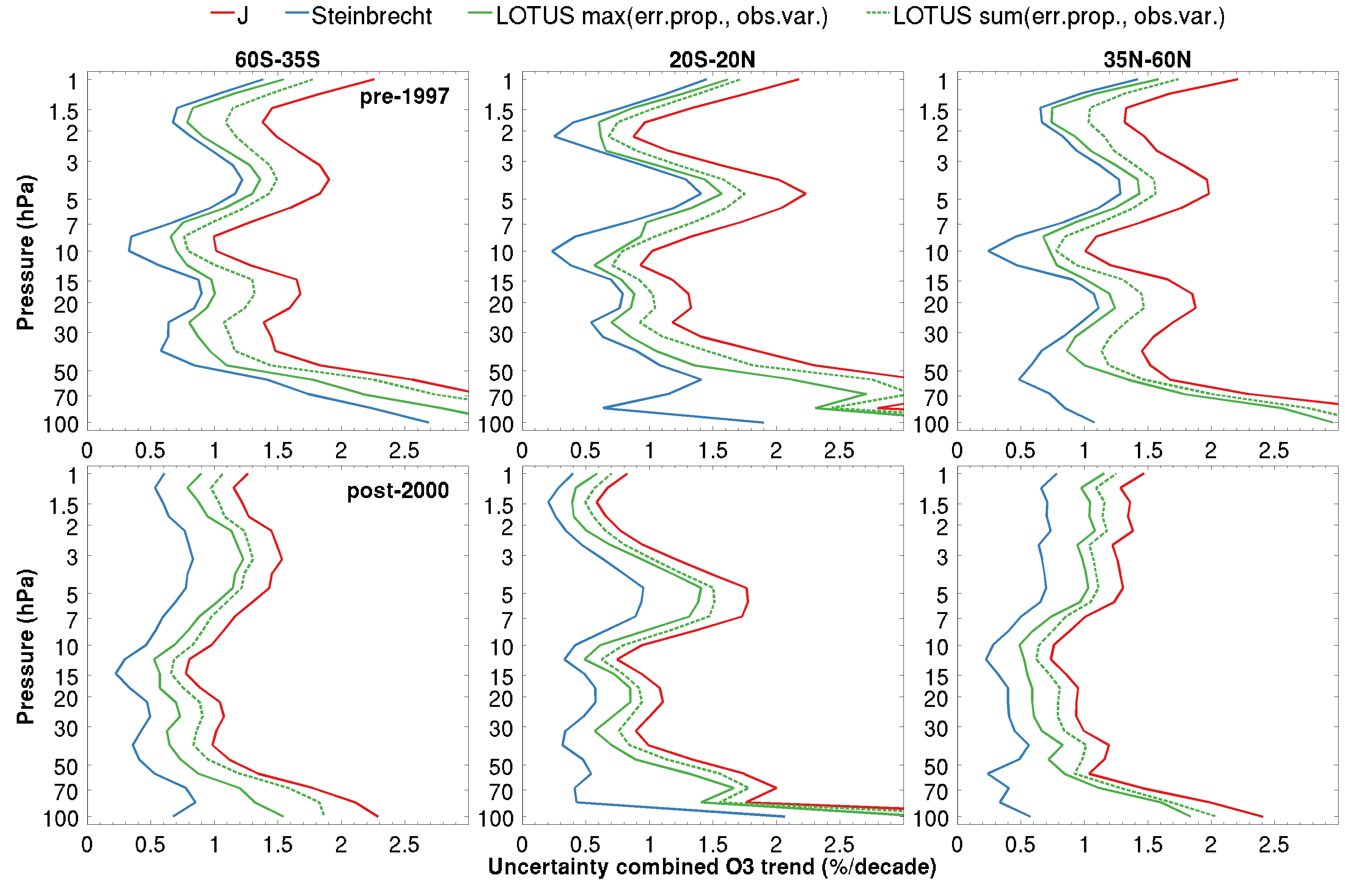	Figure S5.9 | high-res .png Uncertainty (1σ) of combined satellite ILT trends for pre-1997 trends (top) and for post-2000 trends (bottom row). Shown are four methods to compute uncertainty: J-distribution (Equation 5.4), Steinbrecht (Equation 5.5), LOTUS max-method (Equation 5.1) and LOTUS sum-method (Equation 5.1 but max replaced by sum).
	Figure S5.10 | vector .eps | high-res .png Correlation coefficients between the fit residual time series of the SBUV MOD and SBUV COH datasets, as a function of altitude, for two periods in time and three broad latitude bands.
	Figure S5.11 | vector .eps | high-res .png As Figure S5.10, but for the correlation between GOZCARDS and SWOOSH.
	Figure S5.12 | vector .eps | high-res .png As Figure S5.10, but for corr-SAGE-OSIRIS-OMPS and SAGE-CCI-OMPS.
	Figure S5.13 | vector .eps | high-res .png As Figure S5.10, but for SBUV MOD and SAGE-CCI-OMPS.
	Figure S5.14 | vector .eps | high-res .png As Figure S5.10, but for SBUV MOD and GOZCARDS.
	Figure S5.15 | vector .eps | high-res .png As Figure S5.10, but for GOZCARDS and SAGE-CCI-OMPS.